AMAP Conventions Reference

Page Info

• Audience: Beginner to Advanced

• Prerequisites: MTG Reconstruction Tutorial

• Time: 25 minutes

• Output: Full list of MTG variables, reconstruction options, and alias rules

This page is the practical reference for AMAP-style reconstruction from an MTG.

After the tutorial, users usually want to answer three questions:

1. Which columns can I put in my MTG?

2. Which of these columns are worth measuring first?

3. Which Julia options can I change when the default reconstruction is not enough?

This page answers those questions in that order. It is more detailed than the quickstart, but it is still meant to help you make choices, not just to list internal names.

If you have not used AMAP-style reconstruction yet, start here first:

• MTG Reconstruction Tutorial

This page focuses on which MTG columns PlantGeom can read and which reconstruction options exist. The detailed choice of explicit_coordinate_mode is handled on the next page: Explicit Coordinates: Which Option Should I Use?.

The default AMAP-style reconstruction call is:

set_geometry_from_attributes!(
    mtg,
    prototypes;
    convention=default_amap_geometry_convention(),
)

How To Read This Page

If you are new to PlantGeom, read this page in this order:

1. Measurement strategy: decide what you want to measure in your MTG.

2. MTG columns: see which columns PlantGeom can read automatically.

3. Julia options: change behavior with AmapReconstructionOptions(...) only if needed.

4. Alias tables: use them only when your imported column names differ from the defaults.

If your question is specifically about which explicit-coordinate mode to choose, read the next page after this one: Explicit Coordinates: Which Option Should I Use?.

Before the Full Reference: What Should I Actually Measure?

You do not need to measure every variable listed on this page.

In practice, most users fall into one of these three workflows:

Your goal	Measure first	Usually enough?	Notes
Get a first recognizable 3D plant quickly	Length, Width, Thickness	yes for simple synthetic or regular plants	all organs reuse a prototype shape and are mainly distinguished by size
Reconstruct a measured plant with realistic attachment and orientation	previous columns + Offset, insertion angles, optionally Euler angles	yes for many MTGs	this is the standard AMAP-style workflow
Reconstruct from digitized 3D coordinates	explicit coordinates (XX, YY, ZZ, optionally EndX, EndY, EndZ) plus size columns	yes when coordinates are trusted	use AmapReconstructionOptions(explicit_coordinate_mode=...)

If you are unsure where to start, use the second workflow. It is the most broadly useful one.

MTG columns vs Julia options

There are two different things on this page:

• MTG columns are attributes stored on the nodes themselves, such as Length, Width, Offset, or YInsertionAngle.

• Julia options are not stored in the MTG. They are passed once when calling reconstruction.

opts = AmapReconstructionOptions(
    explicit_coordinate_mode=:topology_default,
)

set_geometry_from_attributes!(
    mtg,
    prototypes;
    convention=default_amap_geometry_convention(),
    amap_options=opts,
)

This distinction matters:

• if you want to describe one specific organ, add or change an MTG column on that node

• if you want to change how PlantGeom interprets many nodes, use a Julia option

1. What Can I Measure in My MTG?

1.1 Smallest useful set

Use this set when you mainly want a size-driven reconstruction.

PlantGeom will take a normalized prototype for each organ type and scale it from these values.

Variable	Meaning	Recommended?
Length	organ length	yes
Width	organ width	yes
Thickness	organ thickness	recommended

With only these variables, PlantGeom can already scale a reusable organ shape.

1.2 Standard reconstruction set

Use this set when you want a botanically structured reconstruction from topology and measurements.

This is the set most users should aim for first.

Variable	Meaning	Recommended?
Offset	position of a :+ organ along its bearer	yes for attached organs
XInsertionAngle, YInsertionAngle, ZInsertionAngle	organ orientation at attachment	yes when measured
XEuler, YEuler, ZEuler	local pose correction after insertion	optional
BorderInsertionOffset	lateral shift on bearer cross-section	optional
Phyllotaxy	fallback azimuth when insertion angle data are missing	optional

This is the most common workflow for measured MTGs.

1.3 Explicit-coordinate set

Use this set when your upstream source already provides 3D coordinates, for example from digitizing, scanning, or another reconstruction pipeline.

These columns are powerful, but they are also the easiest ones to misuse if you mix them with topology-based expectations. If you are not sure, stay with the standard set above.

This page only lists the columns. The precise meaning of explicit_coordinate_mode is explained on the next page.

Variable	Meaning	Use when
XX, YY, ZZ	explicit start position	geometry source already provides 3D coordinates
EndX, EndY, EndZ	explicit end position	segment endpoints are known

Use these variables only if your data source already gives coordinates or if you deliberately want coordinate-driven reconstruction.

1.4 Advanced optional variables

These variables are usually not the first thing to measure. They are useful when you already have a working reconstruction and want to make it more faithful or more constrained.

Variable family	Purpose
InsertionMode, BorderInsertionOffset	cross-section insertion behavior
Azimuth, Elevation	world-space orientation stages
DeviationAngle, Orthotropy, StiffnessAngle	biomechanical / architectural bending stages
Plagiotropy, NormalUp	projection/orientation constraints
GeometricalConstraint	clamp direction into a geometric domain
OrientationReset / Global	reset inherited frame

2. Which Reconstruction Options Exist?

These options are not MTG columns. They are Julia options passed to the reconstruction call:

opts = AmapReconstructionOptions(...)

set_geometry_from_attributes!(
    mtg,
    prototypes;
    convention=default_amap_geometry_convention(),
    amap_options=opts,
)

Most users only need to know these first:

Option	What it changes	Default
explicit_coordinate_mode	how XX/YY/ZZ and endpoints are interpreted	:topology_default
verticil_mode	sibling angular spread when azimuth is missing	:rotation360
order_override_mode	whether order maps override present values or only fill missing ones	:override
insertion_y_by_order	default Y insertion angle by branching order	empty
phyllotaxy_by_order	default phyllotaxy by branching order	empty

Recommended mental model:

• first, put the organ-specific measurements in the MTG

• then, only if the reconstruction still does not match your data source, change one of these Julia options

For most projects:

• keep explicit_coordinate_mode=:topology_default unless your coordinate source clearly requires another mode

• keep verticil_mode=:rotation360 unless sibling spread is already fully measured

• keep order_override_mode=:override only when you really want branch-order calibration to dominate node values

If you need to decide between :topology_default, :explicit_rewire_previous, and :explicit_start_end_required, continue with Explicit Coordinates: Which Option Should I Use? after this page.

Common reconstruction recipes

If your plant data looks like...	Put these in the MTG	Usually set these options	Why
simple measured axes and leaves	Length, Width, Thickness, Offset, insertion angles	none	this is the standard topology-driven workflow
same as above, but some local twist/roll is missing from prototypes	previous columns + XEuler, YEuler, ZEuler only where needed	none	Euler angles are best used as local corrections
digitized node positions with trusted start/end coordinates	XX, YY, ZZ, EndX, EndY, EndZ, size columns	explicit_coordinate_mode=:explicit_start_end_required	coordinates should dominate orientation
topology editor control points that should redirect previous segments	XX, YY, ZZ, size columns	explicit_coordinate_mode=:explicit_rewire_previous	explicit nodes act like anchors instead of visible segments
incomplete angle data, but branch order is known	size columns, topology columns, measured angles when available	insertion_y_by_order, phyllotaxy_by_order, maybe order_override_mode=:missing_only	branch-order rules fill or override missing architecture

3. Detailed Variable and Alias Reference

This section is the exact reference for what PlantGeom accepts by default.

You do not need to memorize these tables. Use them when:

• you are importing data and a column is not being recognized

• you want to understand which aliases are accepted out of the box

• you want to build a custom GeometryConvention from the default one

The phrase "first matching alias wins" means that PlantGeom checks the names in order and uses the first one it finds on the node.

3.1 Geometry Convention (default_amap_geometry_convention())

These aliases describe the usual organ-local measurements: size, angles, and explicit translation.

Scale columns

Semantic meaning	Alias lookup order	Default
Length	Length, length, L, l	1.0
Width	Width, width, W, w	1.0
Thickness	Thickness, thickness, Depth, depth	Width value

Angle columns

Semantic meaning	Alias lookup order	Frame	Unit default	Default
X insertion	XInsertionAngle, x_insertion_angle, xinsertionangle	Local	deg	0
Y insertion	YInsertionAngle, y_insertion_angle, yinsertionangle	Local	deg	0
Z insertion	ZInsertionAngle, z_insertion_angle, zinsertionangle	Local	deg	0
X Euler	XEuler, x_euler, xeuler	Local	deg	0
Y Euler	YEuler, y_euler, yeuler	Local	deg	0
Z Euler	ZEuler, z_euler, zeuler	Local	deg	0

Translation columns

Semantic meaning	Alias lookup order	Default
X translation	XX, xx	0.0
Y translation	YY, yy	0.0
Z translation	ZZ, zz	0.0

3.2 AMAP Options (default_amap_reconstruction_options())

This table lists the option names, related aliases, and defaults used by the AMAP reconstruction controller.

If you are just trying to reconstruct a plant, do not start here. Start from the simpler summary above and come back only when you need to understand a specific option in detail.

Option semantic	Default aliases / values
Insertion mode aliases	InsertionMode, insertion_mode, Insertion, insertion
Phyllotaxy aliases	Phyllotaxy, phyllotaxy, PHYLLOTAXY
Verticil mode	:rotation360
Geometrical constraint aliases	GeometricalConstraint, geometrical_constraint, GeometryConstraint, geometry_constraint
Explicit-coordinate handling mode (explicit_coordinate_mode, alias: coordinate_delegate_mode)	:topology_default (:explicit_rewire_previous, :explicit_start_end_required)
Azimuth aliases	Azimuth, azimuth
Elevation aliases	Elevation, elevation
Deviation aliases	DeviationAngle, deviation_angle
Orthotropy aliases	Orthotropy, orthotropy
Stiffness angle aliases	StiffnessAngle, stiffness_angle
Stiffness source aliases	Stifness, stifness, Stiffness, stiffness
Stiffness tapering aliases	StifnessTapering, stifness_tapering, StiffnessTapering, stiffness_tapering
Stiffness apply aliases	StiffnessApply, stiffness_apply
Stiffness straightening aliases	StiffnessStraightening, stiffness_straightening
Broken-segment aliases	Broken, broken
Plagiotropy aliases	Plagiotropy, plagiotropy
NormalUp aliases	NormalUp, normal_up
Orientation reset aliases	OrientationReset, orientation_reset, Global, global
Endpoint X aliases	EndX, end_x, endx
Endpoint Y aliases	EndY, end_y, endy
Endpoint Z aliases	EndZ, end_z, endz
Allometry enabled	true
Allometry width/height interpolation	true
Allometry terminal default length	1.0
Allometry terminal default width	1.0
Allometry terminal default height	1.0
Order attribute	:branching_order
Auto order compute	true
Order override mode	:override
Insertion-by-order map	empty Dict{Int,Float64}
Phyllotaxy-by-order map	empty Dict{Int,Float64}

3.3 Topology columns (used when XX/YY/ZZ are missing)

These columns matter only when node position is reconstructed from topology instead of from explicit coordinates.

Column	Aliases	Meaning	Default
Offset	Offset, offset	Position along bearer where + organ starts	Bearer Length
Border insertion offset	BorderInsertionOffset, border_insertion_offset, BorderOffset, border_offset	Lateral shift for insertion mode	Depends on mode
Insertion mode	InsertionMode, insertion_mode, Insertion, insertion	CENTER, BORDER (SURFACE alias), WIDTH, HEIGHT	BORDER
Phyllotaxy	Phyllotaxy, phyllotaxy, PHYLLOTAXY	Fallback insertion azimuth when XInsertionAngle is missing	0

First matching alias wins.

4. Parameter Guide for First-Time Users

This section explains the variables in the order users usually encounter them while improving a reconstruction.

Size and scale parameters

Length, Width, and Thickness scale the reference mesh in local coordinates (+X is organ length in AMAP). If Thickness is absent, width is reused, which can make flat organs look unnaturally thick.

Example: changing a leaf from Length=0.20 to Length=0.32 stretches only the local +X axis and increases overlap with neighbors without changing insertion position.

When to use what:

• Use measured organ dimensions when available.

• Keep Thickness explicit for leaves if your reference mesh is not already very thin.

• Use a single fallback width/thickness policy only for synthetic plants or quick debugging.

Insertion angles and Euler angles

Insertion angles define attachment orientation relative to the bearer; Euler angles are post-attachment local refinements.

Example: increasing YInsertionAngle from 35 to 65 lifts a leaf away from the stem axis. Adding ZEuler=20 then twists that leaf around its own axis without changing its insertion anchor.

When to use what:

• Use insertion angles for phyllotaxy/branch architecture.

• Use Euler angles for mesh-pose corrections (twist/roll) after topology is correct.

• Avoid compensating missing insertion data with large Euler rotations, because that breaks architectural meaning.

Explicit coordinates: what the columns do

This page intentionally keeps explicit-coordinate behavior at a practical level.

When XX/YY/ZZ are present, the node has an explicit start position. When those columns are absent, PlantGeom reconstructs position from topology (Offset, insertion mode, bearer frame).

If EndX/EndY/EndZ are also present:

• the node end point is explicit as well

• orientation and effective Length are inferred from (start -> end)

• angle stages are skipped for that node because the segment direction is already known

• Width and Thickness are still used normally

Use this mental model:

• XX/YY/ZZ answer: where does the node start?

• EndX/EndY/EndZ answer: where does the node end?

• topology columns such as Offset answer: where should the node be placed when no explicit coordinates are available?

The remaining decision is what PlantGeom should do when a node has explicit start coordinates but no explicit end coordinates. That is exactly what explicit_coordinate_mode controls, and it is explained on the next page: Explicit Coordinates: Which Option Should I Use?.

Allometry delegate semantics (AMAP core)

PlantGeom now applies AMAP-style allometry preprocessing before geometric stages:

• Missing Width/Height can be interpolated along :< axis neighborhoods.

• If only one of width/height is provided, the other is mirrored.

• If a node has components (:/), measured allometry is propagated to missing component values.

• Component length propagation uses AMAP split-vs-copy behavior: successor-chain components split parent Length; direct (no-succession) components copy parent Length.

• For non-terminal nodes with no measured allometry, size collapses to zero (controller behavior).

• Terminal nodes with missing allometry receive configurable defaults.

• Missing predecessor TopWidth/TopHeight are smoothed from next same-type successor bottom sizes.

• Missing complex-node allometry is accumulated from terminal components (length sum, width max).

AMAP option parameters (practical decisions)

This section is about the options that are easy to see in the output but not always easy to choose from the name alone.

InsertionMode: controls lateral insertion offset on the bearer cross-section.

• CENTER: attach at section center.

• BORDER / SURFACE: project insertion direction to the bearer cross-section and stick to the section border.

• WIDTH: shift along width axis.

• HEIGHT: shift along height axis.

Important: these axes are in the bearer local frame (the bearer reference mesh axes), not in global/world axes.

For default_amap_geometry_convention() (length axis = local +X):

• width axis is local +Y

• height axis is local +Z (same direction as thickness/top-height semantics)

So WIDTH means a lateral shift in local Y, and HEIGHT means a lateral shift in local Z.

Use BORDER/SURFACE for "stick to bearer surface" behavior; use CENTER for neutral attachment; use WIDTH/HEIGHT when organs are known to emerge preferentially on one side of the local cross-section.

verticil_mode: controls sibling spread when XInsertionAngle is missing.

• :rotation360: siblings are distributed around 360 degrees.

• :none: no additional spread term.

Use :rotation360 for whorled/regular sibling insertion with missing azimuth data; use :none if azimuth is already fully defined elsewhere.

order_override_mode with order maps (insertion_y_by_order, phyllotaxy_by_order):

• :override: map values replace present attributes.

• :missing_only: map values fill only missing attributes.

Use :override for strict calibration by branch order. Use :missing_only when measured node-level values must stay authoritative.

StiffnessAngle vs Orthotropy: both bend orientation, but StiffnessAngle takes precedence if both are present.

Use StiffnessAngle when a mechanical bending angle is available; keep Orthotropy as a fallback heuristic.

OrientationReset (Global): resets the orientation basis before insertion/euler stages.

Use it when switching from inherited frame behavior to absolute local interpretation at selected nodes.

NormalUp and Plagiotropy: projection stages applied in this order.

NormalUp is mainly a robustness option for dorsiventral organs (typical leaves): it keeps the organ normal oriented toward world +Z after insertion/euler/bending stages, so leaves are less likely to end up upside-down due to noisy angles.

Practical effect:

• It does not move the insertion point.

• It does not redefine topology.

• It adjusts orientation to keep the organ "up-facing" in world space.

Use NormalUp=true for leaf datasets where adaxial/abaxial flips appear. Add Plagiotropy only if you also need directional projection control in the insertion plane.

Why node_convention.length_axis is critical

node_convention.length_axis defines which local reference-mesh axis is considered the organ main axis.

This affects multiple stages, not just scaling:

• allometry: which axis receives Length

• insertion frame: which direction is considered the organ direction

• bending (Orthotropy/StiffnessAngle): bending axis is derived from this main direction

• projection (NormalUp/Plagiotropy): which columns are treated as direction/secondary/normal

• topology placement defaults: how "along the bearer axis" is interpreted

So if the reference mesh was authored with length on local +Z but the convention says length_axis=:x, orientation and projection can look "wrong" even with correct angle values.

Rule of thumb:

• Use default_amap_geometry_convention() (length_axis=:x) for AMAP-style meshes.

• Use a custom GeometryConvention(..., length_axis=:z) when meshes are authored with length on local +Z.

Stifness / StifnessTapering propagation:

• If a node has a stiffness value and /-linked component children, PlantGeom propagates computed StiffnessAngle values to those components.

• StiffnessApply=false disables this propagation for that node.

• Positive Stifness propagates downward-sign bending angles; negative values propagate upward-sign bending angles.

• StifnessTapering controls the curvature profile (0.5 default when missing).

• StiffnessStraightening (0..1 or 0..100) progressively damps propagated bending after that relative position.

• Broken (0..100) forces downstream component angles to -180 after the break threshold.

What GeometricalConstraint is for

GeometricalConstraint is an envelope rule applied after angle/projection stages to keep an organ direction inside a geometric domain (cone/cylinder/plane families).

Typical use cases:

• constrain synthetic roots to stay inside a soil exploration envelope

• keep generated axes inside a training shape when angle data are sparse/noisy

• enforce directional limits without manually tuning every node angle

Important:

• it is an orientation clamp, not a full collision solver

• it does not move the already computed base insertion point

• for chained :< axes, changing orientation still changes downstream positions through topology

5. Stage Order and Semantics

This is the execution order used by the AMAP-style reconstruction pipeline.

You usually do not need to think about every stage. The main reason to read this section is to understand why one variable seems to override another.

Reconstruction applies stages in this order:

1. Allometry preprocessing (interpolation, propagation, smoothing, complex accumulation).

2. Translation / topology base frame.

3. Endpoint override check (EndX/EndY/EndZ).

4. Insertion angles + insertion mode offset.

5. Azimuth/Elevation world orientation override.

6. Orthotropy/StiffnessAngle bending.

7. DeviationAngle world rotation.

8. Euler stage.

9. Projection stage (NormalUp, then Plagiotropy).

10. Geometrical constraint stage (GeometricalConstraint) for cone/cylinder/plane families.

11. Stiffness propagation stage (Stifness / StifnessTapering) writing StiffnessAngle on / components.

Key rules:

• StiffnessAngle takes precedence over Orthotropy.

• OrientationReset=true resets orientation basis to the AMAP base orientation for that node before insertion/euler stages.

• If both projection flags are enabled, NormalUp is applied before Plagiotropy.

• Geometrical constraint stage only re-orients the local basis; node base position remains topology/translation driven.

• Propagated stiffness angles are written to component children before those children are reconstructed.

• Explicit translation attributes keep the node position explicit; topology-based placement is used only when XX/YY/ZZ are absent.

• When endpoint override is active, angle stages are skipped and node Length is inferred from endpoint distance.

• Allometry preprocessing can write inferred values back to nodes (Length, Width, Thickness, TopWidth, TopHeight) when these are missing.

GeometricalConstraint accepted forms:

• String/Symbol kind: "cone", "elliptic_cone", "cylinder", "elliptic_cylinder", "cone_cylinder", "elliptic_cone_cylinder", "plane".

• Dict/NamedTuple with type (or kind) and optional parameters (primary_angle, secondary_angle, radius, secondary_radius, cone_length, normal, d, origin, axis).

• Parameters can also be provided as node columns using aliases such as ConstraintAngle, ConstraintRadius, ConstraintLength, ConstraintNormalX/Y/Z, ConstraintPlaneD, ConstraintOriginX/Y/Z, ConstraintAxisX/Y/Z.

6. Local vs Global Angles in GeometryConvention

This is an advanced customization section. Read it only if you are defining your own GeometryConvention.

Angle scope is controlled per entry in GeometryConvention.angle_map:

• Local angle (frame=:local): composed as T = T ∘ R.

• Global angle (frame=:global): composed as T = recenter(R, pivot) ∘ T.

Global pivots:

• :origin

• Attribute tuple, e.g. (:pivot_x, :pivot_y, :pivot_z)

• Numeric tuple, e.g. (0.0, 0.0, 0.0)

Minimal example:

base = default_amap_geometry_convention()
leaf_conv = GeometryConvention(
    scale_map=base.scale_map,
    angle_map=[
        (names=[:XInsertionAngle], axis=:x, frame=:local, unit=:deg, pivot=:origin),
        (names=[:YInsertionAngle], axis=:y, frame=:local, unit=:deg, pivot=:origin),
        (names=[:Heading], axis=:z, frame=:global, unit=:deg, pivot=(:pivot_x, :pivot_y, :pivot_z)),
        (names=[:XEuler], axis=:x, frame=:local, unit=:deg, pivot=:origin),
    ],
    translation_map=base.translation_map,
    length_axis=:x,
)

7. Order-Based Defaults and Overrides

This section is useful when you do not have a complete measured angle set and want to inject branch-order rules in a controlled way.

When auto_compute_branching_order=true and no numeric order exists in order_attribute, PlantGeom computes branching_order! automatically.

Then for each node:

• insertion_y_by_order[order] can override YInsertionAngle.

• phyllotaxy_by_order[order] can override the phyllotaxy fallback used when XInsertionAngle is missing.

Override modes:

• :override: map values replace attributes when available.

• :missing_only: map values apply only if the attribute is missing.

Effective fallback for missing XInsertionAngle:

effective_x_insertion = phyllotaxy_effective + verticil_term

• verticil_mode=:rotation360 (default): verticil_term = 360 * rank / total

• verticil_mode=:none: verticil_term = 0

8. Option Impact Examples

The examples below show what the main options actually change in the reconstructed geometry.

Read them selectively:

• InsertionMode if organs attach on the wrong side of the bearer

• verticil_mode if sibling organs all overlap when azimuth is missing

• order overrides if your architecture should differ by branching order

• explicit_coordinate_mode if your MTG contains XX/YY/ZZ or endpoints

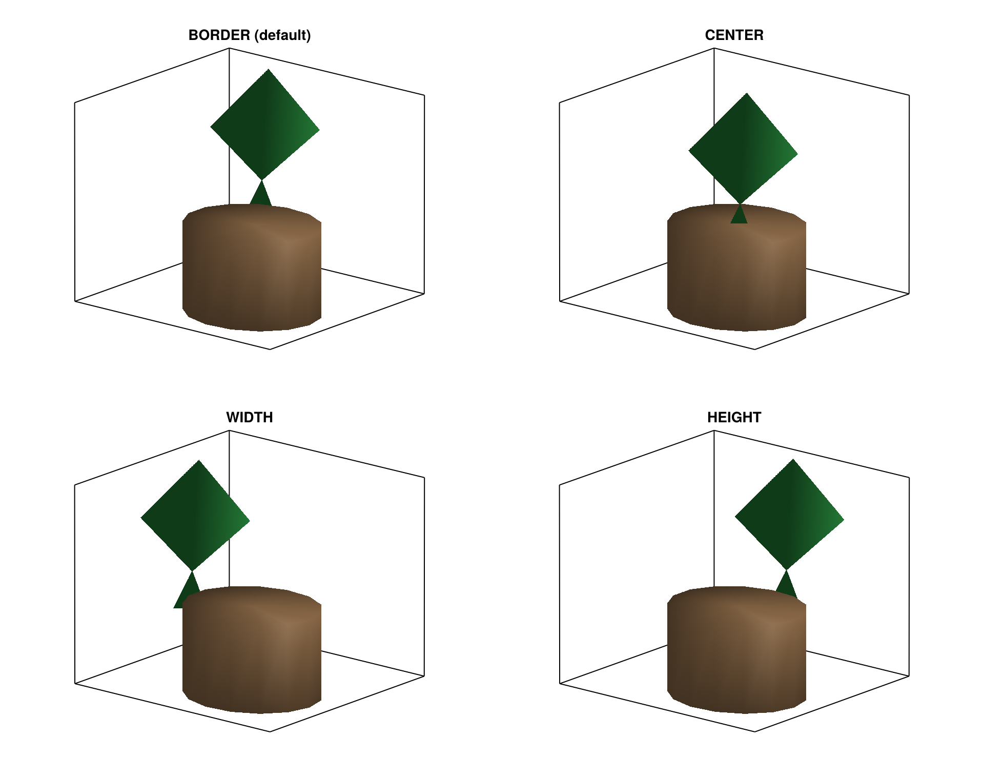
InsertionMode: BORDER (default) vs CENTER vs WIDTH vs HEIGHT

InsertionMode mainly changes where the organ base sits on the bearer cross-section. In practice, this changes self-shading and apparent clumping even if all angles stay identical.

In this example, with AMAP defaults (length=+X) and local frame = reference mesh axes, the distinction is:

• BORDER: offset along the projected insertion direction, to place the organ on bearer surface

• WIDTH: offset along local Y

• HEIGHT: offset along local Z

Use CENTER for symmetric prototypes, WIDTH when organs are known to emerge on lateral flanks, and HEIGHT when emergence is biased toward upper/lower surfaces. If you want "stick to bearer surface" behavior, use InsertionMode="BORDER" (or InsertionMode="SURFACE" alias): this follows insertion direction and projects to the bearer cross-section border.

Why the four panels differ:

• All four cases use the same insertion angles and Offset along the internode.

• Only the lateral insertion direction changes (CENTER = none, BORDER = projected insertion direction, WIDTH = local Y, HEIGHT = local Z).

• So the leaf keeps similar orientation, but its attachment point moves on different cross-section directions.

• In this demo, BorderInsertionOffset is intentionally left missing so defaults are mode-dependent: BORDER -> TopWidth/2, WIDTH -> TopWidth/2, HEIGHT -> TopHeight/2.

• The side can appear left or right depending on orientation because WIDTH/HEIGHT pick +axis or -axis based on alignment with the leaf insertion direction (it is not “always +Y” or “always +Z” in screen space).

Offset and insertion mode are independent:

• Offset: moves the attachment point along the internode axis (+X here).

• BORDER/WIDTH/HEIGHT: move the attachment point across the internode cross-section.

_plot_modes(
    ("BORDER", "CENTER", "WIDTH", "HEIGHT"),
    insertion_mode_example;
    titles=("BORDER (default)", "CENTER", "WIDTH", "HEIGHT"),
    size=(960, 760),
    ncols=2,
    azimuth=1.22pi,
    elevation=0.30,
    zoom_padding=0.035,
)

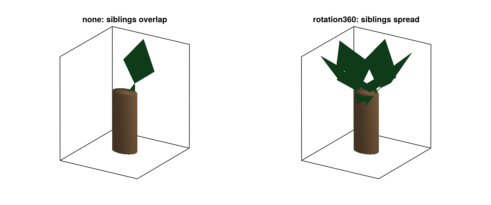
verticil_mode: sibling spread when XInsertionAngle is missing

When insertion azimuth is missing, verticil_mode controls how sibling organs are separated. :rotation360 reduces overlap by design; :none keeps siblings close to the same fallback azimuth.

Use :rotation360 for regular whorls with incomplete azimuth measurements. Use :none if azimuth is already controlled by measured attributes or external rules.

What this figure is doing:

• One internode has 6 sibling leaves.

• Leaves intentionally have no XInsertionAngle (to trigger verticil_mode behavior).

• All siblings share the same Phyllotaxy and YInsertionAngle; only verticil_mode differs.

So the visible difference should be:

• :none: sibling leaves keep the same fallback azimuth and overlap.

• :rotation360: siblings receive an additional spread term (0, 60, 120, ... degrees here), so they form a whorl around the bearer.

To make this easier to see, the demo uses one short bearer with 6 sibling leaves, missing XInsertionAngle, and an eccentric leaf mesh so azimuth spread is visually obvious.

_plot_modes(
    (:none, :rotation360),
    verticil_mode_example;
    titles=("none: siblings overlap", "rotation360: siblings spread"),
    size=(860, 360),
    azimuth=1.18pi,
    elevation=0.38,
    zoom_padding=0.04,
)

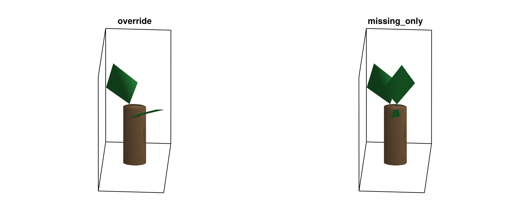
Order-map overrides (:override vs :missing_only)

Order maps are useful for calibrated architecture classes. :override enforces class-level values everywhere; :missing_only preserves measured node attributes and only fills gaps.

Use :override for strict synthetic generators. Use :missing_only for mixed datasets where some organs are measured and others are inferred.

What this specific example does:

• Two leaves share branching_order = 2.

• The order map sets insertion_y_by_order = Dict(2 => 60.0).

• Leaf A has no YInsertionAngle in attributes.

• Leaf B has a measured YInsertionAngle = 15.0.

So the visible difference is:

• :override: both leaves use 60.0, giving a symmetric high insertion posture.

• :missing_only: Leaf A uses 60.0, Leaf B keeps 15.0, giving a clearly asymmetric pair.

_plot_modes(
    (:override, :missing_only),
    order_override_example;
    size=(860, 360),
    azimuth=1.02pi,
    elevation=0.44,
    zoom_padding=0.045,
)

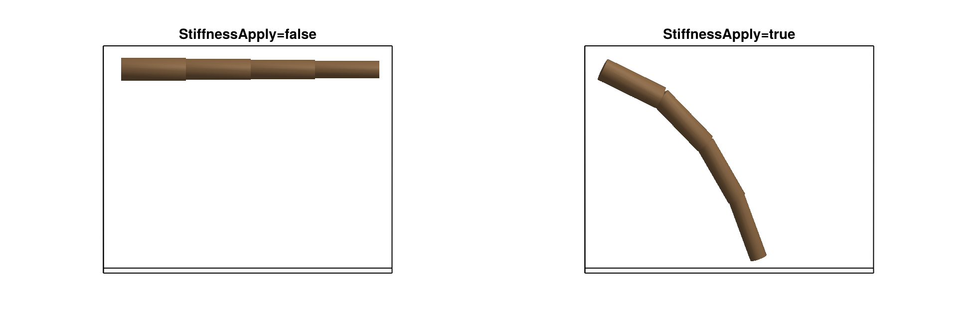
Stiffness propagation (StiffnessApply=false vs true)

This option controls whether node-level Stifness/StifnessTapering are converted into propagated StiffnessAngle values for /-linked component children.

Important: this is a component-based bending mechanism. A single undecomposed reference mesh will not be smoothly bent by this stage; you need a segmented organ representation (explicit per-segment nodes).

What this figure is doing:

• Each controller node has stiffness (Stifness, StifnessTapering) and two / components: an invisible anchor + a visible cylindrical segment.

• StiffnessApply=true propagates a non-zero StiffnessAngle to the visible component.

• Successor :< nodes continue from the last component top (AMAPStudio-like behavior), so propagated component bending changes downstream position.

• Only StiffnessApply changes between panels.

Topology sketch:

AxisNode(i)
├─ / AxisDummy   (anchor, hidden)
└─ / AxisSegment (visible)
< AxisNode(i+1) starts at top(AxisSegment)

So the visible difference should be:

• StiffnessApply=false: segments stay aligned.

• StiffnessApply=true: segments bend and the chain goes downward.

Important: like AMAPStudio, bending changes orientation, and topology controls where the next element starts. If you set explicit XX/YY/ZZ, you override this topological positioning.

_plot_modes(
    (:disabled, :propagate),
    stiffness_propagation_example;
    titles=("StiffnessApply=false", "StiffnessApply=true"),
    size=(980, 320),
    azimuth=1.5pi,
    elevation=0.20,
    zoom_padding=0.05,
)

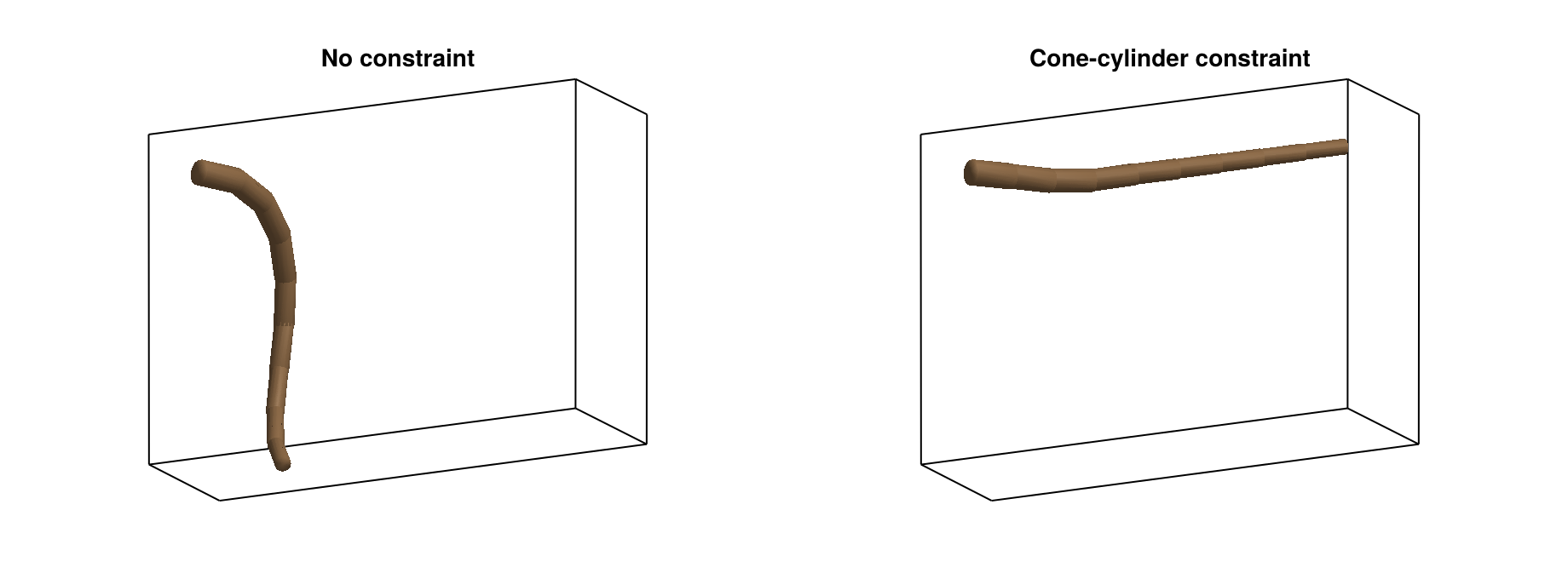
GeometricalConstraint: unconstrained vs constrained axis

This shows the practical role of GeometricalConstraint.

• Left: same insertion/deviation angles, no constraint; the axis drifts away.

• Right: same MTG and angles, with a shared cone_cylinder constraint; directions are clamped and the axis stays inside the envelope.

Use this when you want global shape control (for example root exploration domain) without hand-tuning every segment angle.

_plot_modes(
    (:free, :constrained),
    geometrical_constraint_example;
    titles=("No constraint", "Cone-cylinder constraint"),
    size=(920, 340),
    azimuth=1.35pi,
    elevation=0.26,
    zoom_padding=0.06,
)

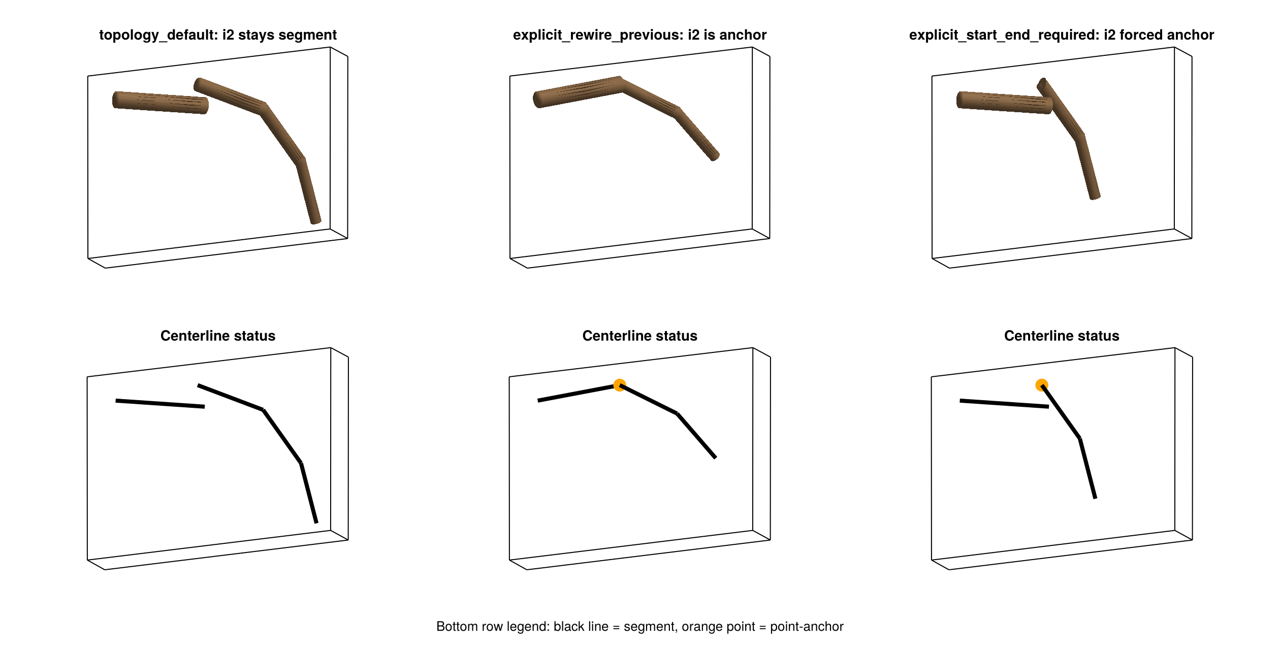
Explicit-coordinate handling mode (explicit_coordinate_mode)

This option controls how explicit start coordinates (XX/YY/ZZ) are used during reconstruction. explicit_coordinate_mode is the recommended API name, and coordinate_delegate_mode is kept as a compatible alias.

In this section, a point-anchor means a node that stays in the MTG but has zero geometric length (a point in space, no cylinder).

What changes between the three panels is mainly the reconstruction rule, not the base MTG. The same 4-internode chain and the same base attributes are used in all cases. The only mode-specific data tweak is for :explicit_start_end_required, where internode 2 is forced to Length=0 with EndX/EndY/EndZ = XX/YY/ZZ so the node stays visible as a point-anchor for side-by-side comparison.

topology_default keeps internode 2 as a normal segment that starts at XX/YY/ZZ. explicit_rewire_previous treats internode 2 as a control point: the previous segment is redirected to this point, and internode 2 itself becomes a point-anchor. explicit_start_end_required applies strict start/end logic: only nodes with a full explicit segment definition can generate a segment.

Use explicit_rewire_previous when you know coordinates for only a few nodes along a long axis. In plain terms, those measured nodes act as waypoints that pull the reconstructed axis toward known positions, while the rest of the axis is still reconstructed from topology and local geometry attributes.

_plot_coordinate_delegate_modes_with_skeleton(
    (:topology_default, :explicit_rewire_previous, :explicit_start_end_required),
    titles=(
        "topology_default: i2 stays segment",
        "explicit_rewire_previous: i2 is anchor",
        "explicit_start_end_required: i2 forced anchor",
    ),
    size=(1260, 640),
    azimuth=1.36pi,
    elevation=0.26,
    zoom_padding=0.065,
)

Numeric interpretation of the same scene (same data, same options):

for mode in (:topology_default, :explicit_rewire_previous, :explicit_start_end_required)
    _print_coordinate_delegate_mode_summary(mode)
end

mode = topology_default
internode | status       | start (x,y,z)        | end (x,y,z)          | length
---------|--------------|----------------------|----------------------|--------
i1       | segment     | (0.0, 0.0, 0.0)      | (0.295, 0.0, -0.052) | 0.3
i2       | segment     | (0.3, 0.06, 0.0)     | (0.518, 0.06, -0.101) | 0.24
i3       | segment     | (0.518, 0.06, -0.101) | (0.644, 0.06, -0.282) | 0.22
i4       | segment     | (0.644, 0.06, -0.282) | (0.695, 0.06, -0.475) | 0.2

mode = explicit_rewire_previous
internode | status       | start (x,y,z)        | end (x,y,z)          | length
---------|--------------|----------------------|----------------------|--------
i1       | segment     | (0.0, 0.0, 0.0)      | (0.3, 0.06, 0.0)     | 0.306
i2       | point-anchor| (0.3, 0.06, 0.0)     | (0.3, 0.06, 0.0)     | 0.0
i3       | segment     | (0.3, 0.06, 0.0)     | (0.491, 0.06, -0.11) | 0.22
i4       | segment     | (0.491, 0.06, -0.11) | (0.619, 0.06, -0.263) | 0.2

mode = explicit_start_end_required
internode | status       | start (x,y,z)        | end (x,y,z)          | length
---------|--------------|----------------------|----------------------|--------
i1       | segment     | (0.0, 0.0, 0.0)      | (0.295, 0.0, -0.052) | 0.3
i2       | point-anchor| (0.3, 0.06, 0.0)     | (0.3, 0.06, 0.0)     | 0.0
i3       | segment     | (0.3, 0.06, 0.0)     | (0.426, 0.06, -0.18) | 0.22
i4       | segment     | (0.426, 0.06, -0.18) | (0.478, 0.06, -0.373) | 0.2

MTG content used in each panel (topology + key attributes):

for mode in (:topology_default, :explicit_rewire_previous, :explicit_start_end_required)
    _print_mode_mtg(mode)
end

mode = topology_default
/Plant1
^/Internode1  Length=0.3  XX=missing  YY=missing  ZZ=missing  EndX=-  EndY=-  EndZ=-  status=segment
^<Internode2  Length=0.24  XX=0.3  YY=0.06  ZZ=0.0  EndX=-  EndY=-  EndZ=-  status=segment
^<Internode3  Length=0.22  XX=missing  YY=missing  ZZ=missing  EndX=-  EndY=-  EndZ=-  status=segment
^<Internode4  Length=0.2  XX=missing  YY=missing  ZZ=missing  EndX=-  EndY=-  EndZ=-  status=segment

mode = explicit_rewire_previous
/Plant1
^/Internode1  Length=0.3  XX=missing  YY=missing  ZZ=missing  EndX=-  EndY=-  EndZ=-  status=segment
^<Internode2  Length=0.24  XX=0.3  YY=0.06  ZZ=0.0  EndX=-  EndY=-  EndZ=-  status=point-anchor
^<Internode3  Length=0.22  XX=missing  YY=missing  ZZ=missing  EndX=-  EndY=-  EndZ=-  status=segment
^<Internode4  Length=0.2  XX=missing  YY=missing  ZZ=missing  EndX=-  EndY=-  EndZ=-  status=segment

mode = explicit_start_end_required
/Plant1
^/Internode1  Length=0.3  XX=missing  YY=missing  ZZ=missing  EndX=missing  EndY=missing  EndZ=missing  status=segment
^<Internode2  Length=0.0  XX=0.3  YY=0.06  ZZ=0.0  EndX=0.3  EndY=0.06  EndZ=0.0  status=point-anchor
^<Internode3  Length=0.22  XX=missing  YY=missing  ZZ=missing  EndX=missing  EndY=missing  EndZ=missing  status=segment
^<Internode4  Length=0.2  XX=missing  YY=missing  ZZ=missing  EndX=missing  EndY=missing  EndZ=missing  status=segment