One Tree, Two Input Files​#

This tutorial reads the same small tree from a plain .vox file and from the merged .jsonl.gz format. Both contain exactly the same plant area density (PAD) on an 8 × 8 × 9 grid. The JSONL file additionally identifies the tree and separates leaf and wood point fractions. We use those fractions to assign optical properties and report leaf absorption separately from wood absorption.

The files are bundled in examples/voxel_tree. The terrain PLY uses the same surface as the interactive tree view.

Download the PAD-only .vox, individual/organ .jsonl.gz, and terrain .ply, or use the copies installed with the package. Together these three files occupy about 24 KiB.

• One Tree, Two Input Files
• Read And Inspect The Files
• Check That The File Format Alone Changes Nothing
• Assign Leaf, Wood, And Individual Properties
• Ground Materials
• Run Both Workflows With Scattering
• Query Vegetation And Ground
• View The Tree And Its Absorption Budget
• Apply The Workflow To Your Data

Read And Inspect The Files​#

using ArchimedLight

example_dir = joinpath(pkgdir(ArchimedLight), "examples", "voxel_tree")
plain_scene = read_scene(joinpath(example_dir, "tree.vox"))
mixed_scene = read_scene(joinpath(example_dir, "tree.jsonl.gz"))
grid = plain_scene.grid
input = mixed_scene.input

@assert grid.minimum == input.grid.minimum
@assert grid.maximum == input.grid.maximum
@assert grid.pad == input.grid.pad

display(plain_scene)
display(mixed_scene)

The plain file already contains a voxelized density field that would be the result of a voxelization process. It supports generic-material interception without any knowledge of which voxel contains the tree or even the partitionning between wood and leaf.

The JSONL reader retains the same density field plus the exported individual and organ proportions.

At the REPL, entering either returned object displays a compact scene summary. Use display(mixed_scene) inside a script to request that summary explicitly; readers do not print during file loading.

Read the independent terrain in the same coordinate frame:

soil = opaque(par=0.12, nir=0.32)
terrain = read_ply_terrain(joinpath(example_dir, "terrain.ply"))
add_ground!(plain_scene, terrain)
add_ground!(mixed_scene, terrain)
(triangles=terrain_patch_count(terrain), bounds_m=terrain_bounds(terrain))

The PLY reader imports geometry and patch identities. Soil reflectance is assigned later in the same model configuration as the vegetation materials.

Without a terrain file, use add_ground!(plain_scene) instead. This creates flat ground at the voxel domain bottom, covering its full x/y extent. See flat ground without a terrain file for patch resolution and elevation options; the default is a geometric assumption rather than an estimated MNT.

Check That The File Format Alone Changes Nothing​#

This synthetic example takes positive y as geographic north and uses scene_rotation_deg=0.0. For measured AMAPVox inputs, check the final scene frame and the distinction between grid and geographic north before choosing the rotation; see Coordinates, Grid North And Scene Rotation.

First give every component the same black material and the same projection coefficient. The plain PAD calculation and the individual/organ calculation must then intercept the same amount of radiation in every voxel.

black = VoxelMaterial(g=0.5)
baseline_scene = VoxelScene(input; terrain)
baseline_models = models_for(;
    mode=:point_proxy, leaf=black, wood=black, unknown=black, ground=soil,
)
plain_baseline_models = models_for(; leaf=black, ground=soil)
row = (
    step_duration=3600.0,
    Ri_PAR_f=100.0,
    Ri_NIR_f=50.0,
    sun_azimuth=180.0,
    sun_elevation=35.0,
    direct_fraction=0.5,
)
first_options = LightOptions(
    toricity=false, scattering=false, turtle_sectors=6, all_in_turtle=true,
    scene_rotation_deg=0.0,
)
backend = VoxelCPUBackend(g=0.5, rays_per_voxel=4)

plain_first = run_light(plain_scene, row; models=plain_baseline_models,
    options=first_options, backend)
mixed_first = run_light(baseline_scene, row; models=baseline_models,
    options=first_options, backend)
@assert isapprox(
    plain_first.first_order.par_energy,
    mixed_first.light.first_order.par_energy;
    rtol=1e-12,
)
@assert isapprox(
    plain_first.first_order.nir_energy,
    mixed_first.light.first_order.nir_energy;
    rtol=1e-12,
)
(same_PAD=grid.pad == input.grid.pad, same_interception=true)

Reading JSONL does not add or remove plant area. Any difference below comes from the declared material assumptions and energy allocation.

Assign Leaf, Wood, And Individual Properties​#

Define default materials once. leaf, wood, and unknown apply to every individual, and ground applies to every soil patch unless an override is supplied. Wood must have zero transmittance, but can reflect intercepted light.

leaf = VoxelMaterial(
    g=0.5,
    par_reflectance=0.08, par_transmittance=0.07,
    nir_reflectance=0.45, nir_transmittance=0.40,
)
wood = VoxelMaterial(
    g=0.5,
    par_reflectance=0.10,
    nir_reflectance=0.30,
)
unknown = VoxelMaterial(g=0.5)

models = models_for(; mode=:point_proxy, leaf, wood, unknown, ground=soil)
@assert isempty(check_models(mixed_scene, models).errors)
models

The example has one individual: numeric tree_id=1 in the file remains integer ID 1 for model lookup and output queries. To modify only this tree's leaf NIR reflectance, supply a partial override:

individual_models = models_for(;
    mode=:point_proxy, leaf, wood, unknown, ground=soil,
    individuals=Dict(1 => (leaf=(nir_reflectance=0.40,),)),
)

A partial named tuple inherits every omitted parameter from the global organ material. Here tree 1 keeps the default leaf PAR coefficients, NIR transmittance and g; its wood and unknown material also stay unchanged. A complete VoxelMaterial instead replaces that organ's whole material. Use the same pattern for several IDs in a multi-tree file. IDs absent from the input are rejected, and a plain .vox file cannot use individual overrides because it contains no individual identities.

You can also provide materials entirely by individual, without a global leaf default. Each positive leaf component then needs a complete material for its individual:

individual_only_models = models_for(;
    mode=:point_proxy, ground=soil,
    individuals=Dict(1 => (leaf=leaf, wood=wood)),
)
isempty(check_models(mixed_scene, individual_only_models).errors)

A partial named tuple needs the corresponding global organ default to inherit from; it cannot fill missing coefficients on its own. Wood and unknown defaults remain black unless supplied or explicitly set to nothing. Missing materials for positive components produce a validation error.

Ground Materials​#

ground_materials assigns soil models to the terrain's material IDs. These IDs belong to geometry and are independent of tree IDs. Define the default soil with the same opaque helper used for triangle materials, then override selected regions in the voxel model configuration:

regional_scene = VoxelScene(grid)
add_ground!(regional_scene; cells=(2, 1), material_ids=reshape([1, 2], 2, 1))
regional_models = models_for(;
    leaf, ground=soil,
    ground_materials=Dict(2 => (par=0.20,)),
)
isempty(check_models(regional_scene, regional_models).errors)

Region 1 uses soil; region 2 changes only par and inherits nir from that global default. A complete opaque(par=..., nir=...) model can replace a region's whole material. opaque fixes transmission to zero; par and nir are reflectances and the absorbed fraction is 1 - reflectance. opaque has no transparency keyword. A translucent model, even with transparency=0, is not accepted for voxel ground. The configuration copies the band coefficients; later edits to the original TypeModel do not change these voxel models.

Run this regional scene and query absorbed PAR for each soil material:

regional_result = run_light(regional_scene, row; models=regional_models,
    options=first_options, backend)
light_metric_values(regional_scene, regional_result, :Ra_PAR_0_q;
    domain=:ground, reduce=sum, by=:material_id)

To omit a global ground default, provide a complete soil model for every material ID used by the terrain:

regional_only_models = models_for(;
    leaf,
    ground_materials=Dict(
        1 => soil,
        2 => opaque(par=0.20, nir=0.32),
    ),
)
isempty(check_models(regional_scene, regional_only_models).errors)

ground_materials is specific to voxel terrain. In a triangle scene, assign that same soil model through its geometry's group and type instead. For ground labelled group="soil", type="ground":

triangle_ground_models = models_for("soil" => ("ground" => soil,))
typeof(triangle_ground_models)

Both ground workflows use outward-hemisphere reflection. For triangles, opaque supports terrain made of nonvertical facets; normals are oriented upward independently of input winding. The geometry must describe terrain, not a closed solid or arbitrary opaque leaf/wood mesh. Triangle translucent plant models retain the existing equal diffuse reflection/transmission split.

The example changes only band optics. To change extinction, set a component's VoxelMaterial.g; this changes the projection hypothesis as well as the calculation. For a VoxelVegetation, the backend's g is an internal positive reference, rather than the place to set individual projection coefficients.

Run Both Workflows With Scattering​#

For plain PAD, assign one homogeneous material to every non-empty cell. Here we deliberately use the default leaf optics everywhere: the plain file cannot identify the lower woody column or the wood fraction in the crown.

options = LightOptions(
    first_options;
    scattering=true,
    scattering_max_iter=30,
    scattering_stop_ratio=1e-8,
)
plain_models = models_for(; leaf, ground=soil)
plain_result = run_light(plain_scene, row; models=plain_models, options, backend)
mixed_result = run_light(mixed_scene, row; models=individual_models, options, backend)
components = component_values(mixed_result; level=:individual)
components

The individual override above changes only leaf NIR reflectance. We can check its effect against the default materials without changing the source file:

default_result = run_light(mixed_scene, row; models, options, backend)
(
    default_NIR_absorbed_J=sum(default_result.light.scattering.nir.absorbed_energy),
    modified_NIR_absorbed_J=sum(mixed_result.light.scattering.nir.absorbed_energy),
    PAR_unchanged=isapprox(default_result.light.scattering.par.absorbed_energy,
                          mixed_result.light.scattering.par.absorbed_energy),
)

Component records aggregate across voxels by individual and organ. Energy fields are joules per step, while plant_area is equivalent proxy area in square metres. Only absorbed PAR of leaf components is leaf APAR; wood absorption belongs to the energy balance but is not photosynthetic absorption. The generic result reports absorbed energy for its homogeneous participating material, without distinguishing those organs.

Query Vegetation And Ground​#

Use the shared metric query to select a tree and organ, or group all individual/organ contributions. These queries preserve the allocation inside shared voxels rather than attributing the whole voxel to every tree:

leaf_apar = light_metric_values(mixed_scene, mixed_result, :Ra_PAR_q;
    individual_id=1, organ=:leaf, reduce=sum)
wood_absorbed = light_metric_values(mixed_scene, mixed_result, :Ra_PAR_q;
    individual_id=1, organ=:wood, reduce=sum)
individual_budget = light_metric_values(mixed_scene, mixed_result, :Ra_PAR_q;
    reduce=sum, by=(:individual_id, :organ))
individual_budget

The default domain is vegetation. Query ground patches explicitly to obtain their incident or absorbed light with the same selectors:

soil_budget = light_metric_values(mixed_scene, mixed_result, :Ra_PAR_q;
    domain=:ground, reduce=sum, by=:material_id)
vegetation_absorbed = light_metric_values(mixed_scene, mixed_result, :Ra_PAR_q;
    reduce=sum)
(
    tree_leaf_APAR_J=leaf_apar,
    tree_wood_PAR_absorbed_J=wood_absorbed,
    initial_vegetation_PAR_absorbed_J=sum(components.Ra_PAR_0_q),
    whole_scene_PAR_absorbed_J=vegetation_absorbed + sum(soil_budget.value),
)

Ground rows contain patch_id, material_id and surface_area; use patch_id= or material_id= to restrict them. Ground fluxes are normalized by the stored patch surface area and step duration. Vegetation fluxes use proxy plant area. Sum energies for a scene budget; use component_values(mixed_result; level=:individual) for area-weighted individual/organ fluxes. The wide component table includes initial and total PAR/NIR incident and absorbed energy/flux, plus Ra_SW_f and aPPFD.

IDs retain their input type: this scene uses Int, so filter with individual_id=1. A separate scene may use text IDs such as "oak-A"; mixed integer and text IDs are rejected, and model keys and query filters must match the scene's ID type. individual_id=(nothing,) selects unattributed vegetation; this synthetic example has none. Organs are :leaf, :wood or :unknown. Voxel coordinate filters and a where row predicate can further restrict a vegetation selection.

View The Tree And Its Absorption Budget​#

The left view shows a front cutaway of the common PAD geometry, coloured by density: the narrow lower column has lower PAD than the crown. The cutaway is only a viewing option; both input files and all calculations retain the full tree. The right view compares vegetation absorption over the same hour: the generic-material result has no organ split; JSONL permits leaf and wood accounting. These illustrative materials do not make either run a calibrated prediction.

using CairoMakie

figure = Figure(size=(1000, 450))
tree_axis = Axis3(
    figure[1, 1]; title="Same tree and terrain (front cutaway)",
    xlabel="x (m)", ylabel="y (m)", zlabel="z (m)",
    aspect=:data, azimuth=-0.86, elevation=0.40, perspectiveness=0.35,
)
lightplot!(
    tree_axis, grid, terrain;
    colormap=[RGBAf(0.43, 0.25, 0.10, 1), RGBAf(0.56, 0.36, 0.12, 1),
        RGBAf(0.57, 0.74, 0.27, 1), RGBAf(0.27, 0.58, 0.19, 1),
        RGBAf(0.07, 0.35, 0.12, 1)],
    colorrange=(0.3, 1.7),
    cutaway=:front, transparency=false,
    voxel_alpha=1.0, voxel_gap=0.1, terrain_alpha=1.0,
    show_lattice=false, show_rays=false, show_normals=false,
    terrain_colormap=[RGBf(0.85, 0.80, 0.70), RGBf(0.85, 0.80, 0.70)],
    terrain_wireframe_color=(:black, 0.12),
    terrain_colorrange=(0.0, 0.4),
)
budget_axis = Axis(
    figure[1, 2]; title="Absorbed PAR in vegetation",
    ylabel="Energy per step (kJ)",
    xticks=([1, 2], ["Generic PAD", "Individual + organs"]),
)
generic_absorbed = sum(plain_result.scattering.par.absorbed_energy) / 1000
barplot!(budget_axis, [1], [generic_absorbed]; color=:slategray, width=0.6)
barplot!(budget_axis, [2], [leaf_apar / 1000]; color=:forestgreen, width=0.6)
barplot!(
    budget_axis, [2], [(leaf_apar + wood_absorbed) / 1000];
    fillto=leaf_apar / 1000, color=:sienna, width=0.6,
)
Legend(
    figure[2, 1:2],
    [PolyElement(color=:slategray), PolyElement(color=:forestgreen), PolyElement(color=:sienna)],
    ["Generic material", "Leaves (APAR)", "Wood"];
    orientation=:horizontal,
)
figure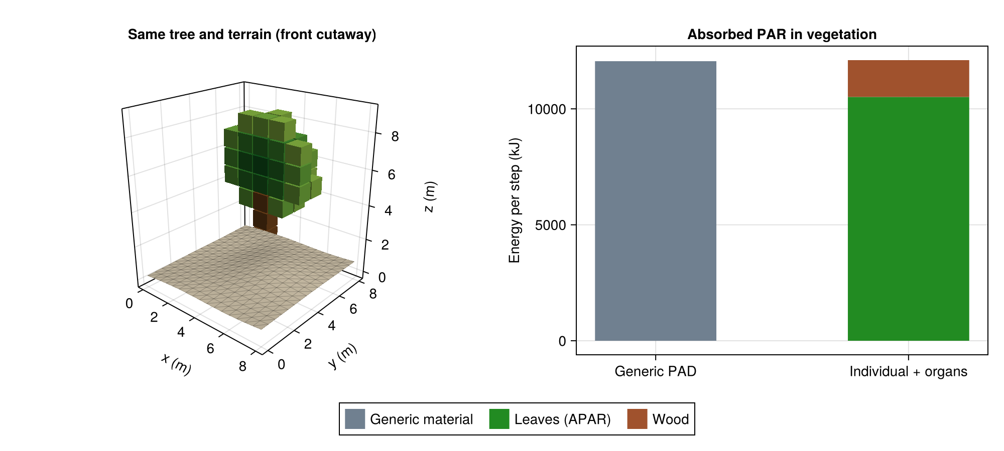

Different optics redistribute scattered radiation, so total absorbed energy can differ even though the initial PAD and projection coefficients are identical. First-order interception remains identical here because every component has g=0.5. Leaf APAR also excludes the wood share that an undifferentiated material cannot identify.

Apply The Workflow To Your Data​#

Replace the example paths with your .vox or merged .jsonl.gz and terrain PLY. A .vox file is sufficient for a generic PAD calculation. Use the JSONL when individual/organ information is available, and keep its optical parameters in the model rather than editing observational input values.

For changing PAD over time, see Successive PAD Files: create a denser second .vox, run each file over its own meteorological period, and reuse caches within each period.

Unlike this fully labelled synthetic example, real exports can contain positive-PAD cells without identified points. Those remain unattributed unknown-organ vegetation and still intercept light. Unknown PAD requires an explicit handling policy; neither format nor point fractions can recover the missing density. See Input Files And Individuals for those cases, Interception And Assumptions for the point-to-area hypothesis, and Terrain And Soil for PLY coverage and alignment checks.