Scattering And Optical Assumptions

After first-order interception, ARCHIMED can redistribute part of the intercepted energy between scene components through iterative scattering.

The light intercepted by an object can be either absorbed, reflected, or transmitted:

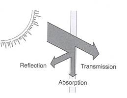
Scattering corresponds to the reflected and transmitted fractions of the intercepted energy. It depends on the optical properties of the component and on the wavelength of the light considered, which are defined in the model files.

In practice, the model takes the energy first intercepted by each object computed during the interception stage (the big band coming from the sun in the figure), applies a waveband-specific scattering coefficient, and redistributes that scattered energy between adjacent visible objects according to hits along the same directional ray paths used for interception.

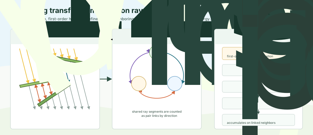
The figure shows the three steps used to turn first-order ray paths into scattering transfers.

For one light direction, and the three components depicted in the figure, the algorithm runs in two main steps:

Step 1: Build the visibility links (panel 1&2)

We shoot many parallel rays from the sky direction through the pixels. Some rays hit the components directly (yellow arrows). This step is the first-order interception stage, which computes the intercepted energy for each component. Then, some light is transmitted or reflected and continues along the ray path (panel 1). Some of those rays hit other components, and some escape to the sky. The algorithm counts how many rays connect each pair of components along the ray path, to tell us who is visible from whom, and how strongly (depending on the number of common rays).

Step 2: Exchange energy (panel 3)

Based on the visibility links (which organ sees which, and how many rays connect them), the algorithm redistributes the scattered energy between components. Each component absorbs part of the energy, and transmits or reflects the rest to its neighbors again. The more rays connect two components, the more energy is exchanged between them. We do this iteratively until the remaining scattered energy in the scene is small enough to stop.

In more detail, panel 3 shows how the graph is used during propagation. A node's current power is multiplied by its scattering coefficient, normalized by the sum of its angularly weighted directional hits, and split between the two transfer sides. Each pair link then receives that share multiplied by its weighted common-hit count, so neighbors receive energy in proportion to their shared ray paths with the source node. The received scattered power becomes part of the next iteration.

An object can also scatter energy toward open sky along one side of a directional path. In that case the energy is treated as leaving the scene: the sky is not added as a receiving node, and no new scattering exchanges are created with it.

How One Scattering Iteration Works

For each node and band:

1. start from the current intercepted or previously scattered energy
2. multiply by the node scattering coefficient
3. divide by the sum of angularly weighted source hits and by two transfer sides
4. multiply that share by each pair link's angularly weighted common-hit count
5. accumulate the resulting received energy on linked neighboring hits
6. treat sky-facing shares with no receiving scene object as escaped energy

The process repeats until the remaining scene-scale scattered energy becomes small enough.

Stopping Rule

The historical ARCHIMED stopping rule is empirical but practical:

current scattered energy <= scattering_stop_ratio × initial scene intercepted energy

The default scattering_stop_ratio = 0.01 means the iteration stops once the remaining scattering pool falls below 1 percent of the initial intercepted energy in the band.

The Main Assumptions

Finite Direction Set

Both incident radiation and scattering exchanges are described over a finite set of discrete directions. The directional discretization is a key assumption of the ARCHIMED method, and it is used for both first-order interception and scattering. The directional set is defined by the turtle sectors, which are built from the meteo step and the sky model.

Lambertian Redistribution

The scattered power follows a discrete Lambertian distribution: outgoing radiance is independent of viewing angle, while power within a solid angle is proportional to the apparent source area. The division by two shares the scattered pool between the two directions along each ray path, retaining the additional assumption of equal reflectance and transmittance.

ARCHIMED rasterizes surfaces on a horizontal ground plane. For a planar component of area A and unit normal n, let s_k be an upward unit turtle direction and s_z,k its vertical component. With the whole projected component inside the projection bounds, the raw directional hit count approximately follows:

H_k ∝ A × |n · s_k| / s_z,k

The projection already encodes the apparent source area. To remove the extra horizontal-plane factor and integrate over solid angle, the graph weights each direction by w_k = s_z,k × sector.weight. Here sector.weight is the sector's normalized solid angle; the common factor 2π cancels during normalization. For source i and receiver j, the transfer per iteration is:

weighted_hits[i] = sum_k(w_k × source_hits[i, k])
weighted_links[j, i] = sum_k(w_k × link_hits[j, i, k])
received[j ← i] = current[i] × scattering_coefficient[i]
                  × weighted_links[j, i] / (2 × weighted_hits[i])

A source with no weighted hits transfers no power. Source totals include rays that escape without hitting another object, so successful links are never renormalized to hide escape. Explicit :sun directions are excluded from this angular quadrature. The weights depend on geometry and sector solid angles, not on the current sky brightness or incident flux. No additional cosine to the source normal is applied: it is already present in the hit count.

For a horizontal surface this gives power proportional to s_z,k × ΔΩ_k; for an inclined surface it gives |n · s_k| × ΔΩ_k. This is the Lambertian radiometric integral approximated with the selected turtle directions and raster pixels. Finer pixels do not remove errors due to a coarse angular grid. In particular, per-component discrete normalization preserves the scattered power but does not guarantee exact continuum view factors or reciprocity at finite angular resolution.

The historical Java MUSC implementation, and Julia before the issue #55 correction, used unweighted link and source-hit counts. Equal ray energies with horizontal rasterization overrepresented shallow directions, even with fine pixels. The correction implements the technical manual's stated Lambertian assumption and intentionally changes historical scattering results. It retains the simplified optical coefficients and equal two-sided split. Analytical plate tests verify the numerical weighting; they do not replace physical measurements of irradiance within a scene.

Explore the Evaluation page to compare the current algorithm with an independent surface-integral reference in four interactive 3D scenes. It also explains how the reference handles projected area, occlusion, diffuse transmission, and repeated exchanges.

Optical Coefficients

In model files, optical_properties store scattering factors by waveband:

optical_properties:
  PAR: 0.15
  NIR: 0.90

PAR has typically low scattering because most intercepted PAR is absorbed by leaves. Whereas NIR scattering is typically high, meaning much more of the intercepted NIR is re-emitted into the scattering process.

Artificial Light Emitters

Artificial emitters use a separate, cosine-weighted source calculation. Their initial emission is calculated before the subsequent scattering by ordinary surfaces described above.

The light source formalism can be read with three indices: source s, waveband b, and direction d. Natural illumination has sources such as the sun and sky sectors. An artificial emitter adds another source to that same light budget.

For an emitter, radiance is the Lambertian spectral radiance L per emitting surface area and steradian. gamma contains independent waveband coefficients; the values are used exactly as supplied and are not normalized. For a source surface of area A, the hemispherical source power for band b is:

P[b, s] = pi * A[s] * L[s] * gamma[b, s]

The current emitter model is one-sided and assumes horizontal surfaces emitting into the downward hemisphere, which is discretized with the non-solar turtle sectors. Each sector is weighted by both its solid angle and cos(theta); a single quadrature correction preserves the exact Lambertian hemispherical integral pi. Within a sector, emission is uniform per projected source area. A ray is assigned only to its first distinct geometric hit. Another emitting surface is therefore an occluding receiver, while a ray with no subsequent hit is recorded as escaped energy. Receiver shares plus the escaped share equal the emitted power; successful hits are never renormalized to hide escape.

Virtual sensors are observations rather than physical first hits. They record the emitter power crossing their surface, but the ray continues to the first physical receiver or to escape. Sensor observations are consequently not part of the received-plus-escaped energy closure. Custom gamma entries use the same transfer fractions as PAR and NIR and remain separate wavebands throughout first-order interception and scattering.

The historical Java implementation interpreted radiance as component-total power. To reproduce an old Java source with total magnitude P_java on one panel of area A, use L = P_java / (pi * A) in the Julia model. The Java light-source fixtures are retained as numerical regression references through this explicit conversion; they do not override the area-based radiance definition above.

Emitter-contributed first-order light joins the same scattered energy pool as sky and sun light when scattering is enabled.

This is deliberately simpler than a full photometric lamp or point-source ray tracer, but it is sufficient for the purpose of adding artificial light to a scene.

Virtual Sensors

Virtual sensors are special because they receive light and can report how much they receive, but they do not behave as absorbing geometry. In other words, they are treated as transparent during scattering and their scattering coefficient is zero. For Java parity, their observations still enter the scene-wide convergence total. A sensor can therefore affect the finite iteration at which the solver stops when the result lies very close to the stopping threshold, even though the sensor never re-emits or consumes the transferred energy. They usually are used to measure light received at a specific location, such as a sensor on a leaf or a camera in the scene.

Soil And Ground Matter More When Scattering Is Enabled

Without ground geometry, a significant part of the lower-canopy exchange can be missed. That is why it is highly recommended to use paving or explicit ground tiles whenever scattering is active.