Outputs

The current Julia package exposes light results in three increasingly concrete forms:

1. in memory as LightBudget
2. attached back onto MTG nodes as ARCHIMED-style attributes
3. written to disk when you export the enriched scene

This page documents those three layers and then explains the ARCHIMED-style CSV outputs used by the public writer and regression harness.

1. In-Memory Outputs: LightBudget

The core output of run_light for one meteo row is:

using ArchimedLight

repo_root = normpath(joinpath(dirname(pathof(ArchimedLight)), ".."))
config = joinpath(repo_root, "example_2", "config.yml")
sim, meteo = read_simulation(config)
sky_options = LightOptions(sim.options; include_sky_fraction=true)
sim = LightSimulation(sim.scene, sim.models; options=sky_options)
row = first(meteo)
step = run_light(sim, row)
budget = step.budget;

LightBudget(ArchimedLight.InitialTotalSpectralNodeValues(ArchimedLight.SpectralNodeValues(Dict(4986 => 406.8140334585218, 4700 => 348.0794473976367, 4576 => 352.2741612772015, 6073 => 27.90309169241545, 2288 => 40.83070102959615, 1703 => 76.81670769946986, 1956 => 148.33471030074412, 2350 => 89.67606460798676, 5975 => 170.25722270995877, 3406 => 34.06421012226389…), Dict(4986 => 440.7152029133987, 4700 => 377.08606801410656, 4576 => 381.6303413836349, 6073 => 30.228349333450073, 2288 => 44.233259448729164, 1703 => 83.21810000775902, 1956 => 160.69593615913948, 2350 => 97.14906999198566, 5975 => 184.4453246024553, 3406 => 36.902894299119204…)), ArchimedLight.SpectralNodeValues(Dict(4986 => 410.80235212394194, 4700 => 353.6260778162413, 4576 => 356.46037018295107, 6073 => 33.9695357020266, 2288 => 56.077085524614255, 1703 => 97.87440744698361, 1956 => 170.6720370974211, 2350 => 107.82943565589999, 5975 => 174.83834477128153, 3406 => 50.31264134268901…), Dict(4986 => 549.9679365646249, 4700 => 495.25054187133355, 4576 => 493.3441067839269, 6073 => 181.171314723127, 2288 => 451.47749063949055, 1703 => 559.3112801334534, 1956 => 582.4260015532606, 2350 => 526.9681096909218, 5975 => 304.9706025235159, 3406 => 399.4049904371986…))), ArchimedLight.InitialTotalSpectralNodeValues(ArchimedLight.SpectralNodeValues(Dict(4986 => 1512.9453386921832, 4700 => 1294.5129649624198, 4576 => 1310.1123131854213, 6073 => 103.77190283138725, 2288 => 48.101062763319135, 1703 => 75.26075636060305, 1956 => 858.3430896092847, 2350 => 826.0777849822961, 5975 => 633.1868106330966, 3406 => 166.16747669089526…), Dict(4986 => 1639.0241169165322, 4700 => 1402.389045375955, 4576 => 1419.2883392842061, 6073 => 112.41956140066954, 2288 => 52.109484660262396, 1703 => 81.53248605731997, 1956 => 929.8716804100585, 2350 => 894.9176003974875, 5975 => 685.9523781858545, 3406 => 180.0147664151365…)), ArchimedLight.SpectralNodeValues(Dict(4986 => 1527.7779345167855, 4700 => 1315.1409711329081, 4576 => 1325.6808800456895, 6073 => 126.33307437599196, 2288 => 66.06223607202574, 1703 => 95.8919244707055, 1956 => 987.5986769050642, 2350 => 993.3029705518948, 5975 => 650.2240089437455, 3406 => 245.42840205487283…), Dict(4986 => 2045.3360936980666, 4700 => 1841.8445907974565, 4576 => 1834.7533256249517, 6073 => 673.7780986611358, 2288 => 531.868093514601, 1703 => 547.9822195523662, 1956 => 3370.2248963066863, 2350 => 4854.3237341284275, 5975 => 1134.186027911894, 3406 => 1948.324038646156…))), ArchimedLight.InitialTotalSpectralNodeValues(ArchimedLight.SpectralNodeValues(Dict(4986 => 345.7919284397435, 4700 => 295.8675302879912, 4576 => 299.43303708562127, 6073 => 23.717627938553132, 2288 => 34.70609587515673, 1703 => 65.29420154454938, 1956 => 126.0845037556325, 2350 => 76.22465491678875, 5975 => 144.71863930346495, 3406 => 28.954578603924304…), Dict(4986 => 44.07152029133986, 4700 => 37.708606801410646, 4576 => 38.163034138363486, 6073 => 3.0228349333450066, 2288 => 4.423325944872915, 1703 => 8.3218100007759, 1956 => 16.069593615913945, 2350 => 9.714906999198563, 5975 => 18.444532460245526, 3406 => 3.6902894299119198…)), ArchimedLight.SpectralNodeValues(Dict(4986 => 349.18199930535064, 4700 => 300.5821661438051, 4576 => 302.9913146555084, 6073 => 28.874105346722608, 2288 => 47.665522695922114, 1703 => 83.19324632993607, 1956 => 145.07123153280793, 2350 => 91.65502030751499, 5975 => 148.6125930555893, 3406 => 42.765745141285656…), Dict(4986 => 54.99679365646248, 4700 => 49.52505418713334, 4576 => 49.33441067839268, 6073 => 18.117131472312696, 2288 => 45.14774906394904, 1703 => 55.93112801334532, 1956 => 58.242600155326045, 2350 => 52.69681096909217, 5975 => 30.49706025235158, 3406 => 39.94049904371985…))), ArchimedLight.InitialTotalSpectralNodeValues(ArchimedLight.SpectralNodeValues(Dict(4986 => 1286.0035378883556, 4700 => 1100.3360202180568, 4576 => 1113.595466207608, 6073 => 88.20611740667917, 2288 => 40.885903348821266, 1703 => 63.971642906512585, 1956 => 729.591626167892, 2350 => 702.1661172349517, 5975 => 538.2087890381321, 3406 => 141.24235518726096…), Dict(4986 => 163.90241169165319, 4700 => 140.2389045375955, 4576 => 141.92883392842057, 6073 => 11.24195614006695, 2288 => 5.210948466026239, 1703 => 8.153248605731996, 1956 => 92.98716804100583, 2350 => 89.49176003974873, 5975 => 68.59523781858545, 3406 => 18.001476641513648…)), ArchimedLight.SpectralNodeValues(Dict(4986 => 1298.6112443392676, 4700 => 1117.869825462972, 4576 => 1126.828748038836, 6073 => 107.38311321959317, 2288 => 56.15290066122187, 1703 => 81.50813580009968, 1956 => 839.4588753693045, 2350 => 844.3075249691105, 5975 => 552.6904076021837, 3406 => 208.61414174664188…), Dict(4986 => 204.5336093698066, 4700 => 184.1844590797456, 4576 => 183.47533256249514, 6073 => 67.37780986611357, 2288 => 53.18680935146009, 1703 => 54.798221955236606, 1956 => 337.0224896306686, 2350 => 485.43237341284265, 5975 => 113.41860279118936, 3406 => 194.83240386461554…))), Dict{String, Dict{Int64, Float64}}(), Dict{String, Dict{Int64, Float64}}(), Dict("PAR" => Dict(), "NIR" => Dict()))

The main grouped fields are:

• budget.incident_flux
• budget.incident_energy
• budget.absorbed_flux
• budget.absorbed_energy

Each one is then split into:

• initial: first-order interception only
• total: first-order plus scattering

and by waveband, for example:

• par
• nir

Typical accesses:

budget.incident_flux.initial.par;
budget.incident_flux.total.par;
budget.absorbed_energy.total.nir;

Dict{Int64, Float64} with 5968 entries:
  4986 => 204.534
  4700 => 184.184
  4576 => 183.475
  6073 => 67.3778
  2288 => 53.1868
  1703 => 54.7982
  1956 => 337.022
  2350 => 485.432
  5975 => 113.419
  3406 => 194.832
  2841 => 450.693
  2876 => 18.1699
  687  => 353.35
  185  => 496.362
  1090 => 421.839
  2015 => 163.193
  3293 => 296.724
  3220 => 9.82145
  4888 => 182.794
  ⋮    => ⋮

Each leaf of that structure is a dictionary keyed by node id.

For artificial emitters, step.first_order.emitter_escaped_power.par and .nir report emitted power which left the represented scene without a geometric hit. These dictionaries are keyed by emitting source node. Together with emitter-contributed incident power, they provide the explicit received-plus-escaped power closure (in W) described in Artificial Light Emitters. Virtual sensors are non-consuming observations: their reported incident power is not subtracted from the ray and is excluded from this physical received-plus-escaped closure. A sensor may therefore report the same ray that is subsequently received by a physical component or escapes the scene. first_order.incident_power combines artificial emitters with sky and sun sources. To verify the closure from public fields, external sky/sun input must be zero and incident power must be summed over physical (non-sensor) receivers; sensor entries are observations, not consumed power. The emitter transfer is accounted separately before it is merged into total incident power. emitter_escaped_power exposes instantaneous PAR and NIR power. The integrated step budget exposes every emitted band, including custom bands, through step.budget.emitter_escaped_energy_per_band[band]. For PAR and NIR this is the corresponding escaped power multiplied by the step duration in seconds.

If you need canopy-view metadata for coupled models, step.sky_fraction stores the per-node visible-sky fraction when options.include_sky_fraction=true. When using a YAML config, read_options enables that option when component_variables.sky_fraction or opf_variables.sky_fraction is true.

2. Query Values By Scene Metadata

light_metric_values combines a light result with its scene metadata and returns a Tables.jl-compatible column table:

coffee_leaves = light_metric_values(
    sim,
    step,
    :absorbed_par_energy;
    species="coffee",
    object_id=1,
    symbol=:Leaf,
)

propertynames(coffee_leaves)

(:step_number, :node_id, :source_topology_id, :object_id, :item_id, :component_id, :group, :type, :symbol, :scale, :value)

The table includes the timestep, runtime and source node identifiers, object and output grouping identifiers, group/type, MTG symbol and scale, and the selected value. A series produces the same columns in long form:

coffee_series = light_metric_values(
    sim,
    [step],
    :Ra_PAR_q;
    species="coffee",
)

unique(coffee_series.step_number)

1-element Vector{Int64}:
 1

All filters combine. group and species are aliases, object_id identifies one placed scene object, source_topology_id identifies its source component, and node_ids accepts one runtime node id or a collection. symbol, scale, type, exact attributes, and a custom where node predicate provide progressively more specific selection.

Selections can be reused:

leaf_ids = light_node_ids(sim; species="coffee", symbol=:Leaf)
leaf_par = light_metric_values(sim, step, :Ra_PAR_q; node_ids=leaf_ids)
leaf_nir = light_metric_values(sim, step, :Ra_NIR_q; node_ids=leaf_ids)
length(leaf_par.value) == length(leaf_nir.value)

true

Use reduce=sum for a total. For example, these compute the whole-scene absorbed PAR and the plant-only total after excluding paving:

scene_absorbed_par = light_metric_values(
    sim,
    step,
    :absorbed_par_energy;
    reduce=sum,
)

plant_ids = setdiff(
    light_node_ids(sim),
    light_node_ids(sim; group="pavement"),
)
plant_absorbed_par = light_metric_values(
    sim,
    step,
    :absorbed_par_energy;
    node_ids=plant_ids,
    reduce=sum,
)

scene_absorbed_par >= plant_absorbed_par

true

Adding by, such as by=:object_id or by=(:group, :type), returns a grouped table. For a series, step_number is retained automatically. sink=DataFrame can materialize detailed or grouped results when DataFrames.jl is loaded.

Summing per-component energy (*_energy or historical *_q) gives an energy total. Flux values are normalized independently by each component's area, so their direct sum generally is not a meaningful scene-scale flux.

Dynamic scenes

Each result retains a lightweight node metadata snapshot by default. All steps computed without changing the scene share the same snapshot. After update_scene!, the next result receives a new snapshot, allowing one series to contain several runtime node-id layouts safely:

steps = LightStepResult[]
for (new_scene, row) in zip(scenes, meteo)
    update_scene!(sim, new_scene)
    push!(steps, run_light(sim, row))
end

second_coffee_leaf = light_metric_values(
    sim,
    steps,
    :absorbed_par_energy;
    species="coffee",
    object_id=2,
    source_topology_id=42,
)

The stable component identity is normally (object_id, source_topology_id); runtime node_id remains local to one scene version. To retain additional scalar identifiers, construct options with node_metadata_attributes=(:organ_id, ...) and filter with attributes=(organ_id=...,). Set store_node_metadata=false when results are queried immediately and minimum retained memory is more important.

3. Attached Outputs: ARCHIMED Attribute Names

The convenience layer for visual inspection is attach_light_step!:

attach_light_step!(
    sim.scene,
    step;
    fields=[:incident_par_flux, :incident_par_energy, :absorbed_par_energy],
);

/ 1: Scene
├─ / 2: Individual
│  └─ / 3: Axis
│     ├─ / 4: Metamer
│     ├─ < 5: Metamer
│     ├─ < 6: Metamer
│     ├─ < 7: Metamer
│     ├─ < 8: Metamer
│     ├─ < 9: Metamer
│     ├─ < 10: Metamer
│     ├─ < 11: Metamer
│     │  ├─ + 12: Axis
│     │  │  ├─ / 13: Metamer
│     │  │  ├─ < 14: Metamer
│     │  │  ├─ < 15: Metamer
│     │  │  ├─ < 16: Metamer
│     │  │  ├─ < 17: Metamer
│     │  │  ├─ < 18: Metamer
│     │  │  ├─ < 19: Metamer
│     │  │  │  └─ + 20: Axis
│     │  │  │     ├─ / 21: Metamer
│     │  │  │     ├─ < 22: Metamer
│     │  │  │     ├─ < 23: Metamer
│     │  │  │     ├─ < 24: Metamer
…

The default mappings are:

The meaning follows the historical ARCHIMED naming:

• area: prepared object surface area in m^2
• Ri: intercepted radiation
• Ra: absorbed radiation
• _0_: first-order only
• no _0_: after scattering has been added
• _f: irradiance-like quantity in W m^-2
• _q: energy per component and per step in J

You can also rename attached attributes for downstream packages. For example, PlantBiophysics can use Ra_SW_f as an alias for absorbed NIR:

attach_light_step!(
    sim.scene,
    step;
    fields=[:area, :absorbed_par_flux, :absorbed_nir_flux, :sky_fraction],
    names=Dict(:absorbed_nir_flux => :Ra_SW_f),
);

/ 1: Scene
├─ / 2: Individual
│  └─ / 3: Axis
│     ├─ / 4: Metamer
│     ├─ < 5: Metamer
│     ├─ < 6: Metamer
│     ├─ < 7: Metamer
│     ├─ < 8: Metamer
│     ├─ < 9: Metamer
│     ├─ < 10: Metamer
│     ├─ < 11: Metamer
│     │  ├─ + 12: Axis
│     │  │  ├─ / 13: Metamer
│     │  │  ├─ < 14: Metamer
│     │  │  ├─ < 15: Metamer
│     │  │  ├─ < 16: Metamer
│     │  │  ├─ < 17: Metamer
│     │  │  ├─ < 18: Metamer
│     │  │  ├─ < 19: Metamer
│     │  │  │  └─ + 20: Axis
│     │  │  │     ├─ / 21: Metamer
│     │  │  │     ├─ < 22: Metamer
│     │  │  │     ├─ < 23: Metamer
│     │  │  │     ├─ < 24: Metamer
…

4. Disk Outputs: Exported Scenes

Once results are attached, you can export the enriched scene:

scene_path = joinpath(mktempdir(), "scene_with_light.opf")
write_scene(scene_path, sim.scene)
isfile(scene_path)

true

Supported export formats are:

• .ops
• .opf
• .gwa

The export path determines the format.

This is currently the main disk output mechanism of ArchimedLight.jl: attach node attributes, then write the scene back out.

Example Output Images

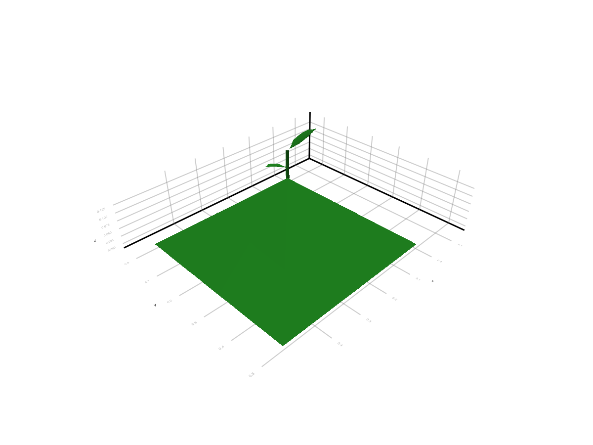
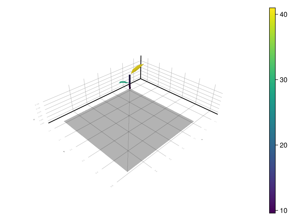
ARCHIMED-Style CSV Tables

The public writer produces component_values.csv. Historical fixture datasets and internal regression tools may also contain files such as:

• component_values.csv
• scene_values.csv
• summary.csv

The example writes a fresh component_values.csv on demand, while the regression and release harnesses under test/ keep their own isolated reference data.

component_values.csv

Component-scale outputs, typically one row per scene node and step. Common columns are:

• step_number
• object_id
• source_topology_id
• group
• type
• area
• Ri_*
• Ra_*

You can write this table from already-computed results:

series = run_light(sim, meteo)
component_path = joinpath(mktempdir(), "component_values.csv")
write_component_values(component_path, sim, series)
isfile(component_path)

true

step_index_base=0 is available for compatibility with historical harness outputs.

scene_values.csv

Scene-scale summary per meteo step.

summary.csv

Grouped aggregation, usually by item, group, and type.

Which Output Form Should You Use

• use LightBudget when staying inside Julia
• use attach_light_step! when you want visual inspection or downstream scene export
• use component_values.csv when you need a portable component-scale table