Getting Started

This page is the shortest path to your first light simulation. It uses the bundled coffee example from example_2/, which is also the source of the image on the home page. Here is how to plot it:

using CairoMakie, PlantGeom

repo_root = normpath(joinpath(dirname(pathof(ArchimedLight)), ".."))
ops_path = joinpath(repo_root, "example_2", "scene", "coffee.ops")
scene_preview = read_scene(ops_path)
plantviz(scene_preview.mtg, color = Dict("Mesh0" => :gray87, "Mesh1" => "#42A25ABD"))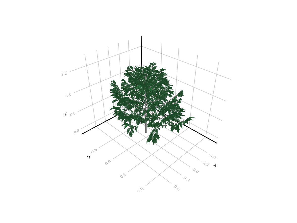

What This Example Covers

reading parameters from files, using a config.yml as the single source of truth for file paths and model options
loading a scene from .ops and .opf
loading functional-group models from YAML
reading one meteo step
running one light step
attaching Ri_PAR_f to the scene for visualization or export

Minimal Run

using ArchimedLight

repo_root = normpath(joinpath(dirname(pathof(ArchimedLight)), ".."))
config = joinpath(repo_root, "example_2", "config.yml")
sim, meteo = read_simulation(config)
scene = sim.scene
models = sim.models
options = sim.options
row = first(meteo)
step = run_light(sim, row)

LightStepResult
  ------------------------------------------------------------
  sky        PAR 463.139 W m^-2  |  NIR 501.734 W m^-2
  sun        azimuth 309.4°  |  elevation 76.5°
  mix        direct 73.5%  |  diffuse 26.5%  |  SW 964.872 W m^-2
  turtle     16 sectors (sky=16, sun=0)
  ------------------------------------------------------------
  incident   PAR 3.724 MJ  |  NIR 9.594 MJ
  absorbed   PAR 3.165 MJ  |  NIR 959.362 kJ
  scattering on  |  iterations 13  |  converged true
  added      PAR 297.823 kJ  |  NIR 5.882 MJ
  ------------------------------------------------------------

The result is a LightStepResult. The most useful field at first is step.budget, which groups values by:

quantity: incident or absorbed
form: flux (W m^-2) or energy (J per component per step)
stage: initial for first-order only, total for first-order plus scattering
waveband: par, nir, and any extra shortwave bands present in the meteo file

Attach Results Back Onto The Scene

ArchimedLight.jl keeps the simulation results in the LightStepResult by default. If you want an inspectable scene, attach selected outputs back onto the MTG:

sky_options = LightOptions(options; include_sky_fraction=true)
sim_with_sky = LightSimulation(scene, models; options=sky_options)
step_with_sky = run_light(sim_with_sky, row)
attach_light_step!(
    scene,
    step_with_sky;
    fields=[:area, :incident_par_flux, :incident_par_energy, :absorbed_par_energy, :sky_fraction],
)

/ 1: Scene
├─ / 2: Individual
│  └─ / 3: Axis
│     ├─ / 4: Metamer
│     ├─ < 5: Metamer
│     ├─ < 6: Metamer
│     ├─ < 7: Metamer
│     ├─ < 8: Metamer
│     ├─ < 9: Metamer
│     ├─ < 10: Metamer
│     ├─ < 11: Metamer
│     │  ├─ + 12: Axis
│     │  │  ├─ / 13: Metamer
│     │  │  ├─ < 14: Metamer
│     │  │  ├─ < 15: Metamer
│     │  │  ├─ < 16: Metamer
│     │  │  ├─ < 17: Metamer
│     │  │  ├─ < 18: Metamer
│     │  │  ├─ < 19: Metamer
│     │  │  │  └─ + 20: Axis
│     │  │  │     ├─ / 21: Metamer
│     │  │  │     ├─ < 22: Metamer
│     │  │  │     ├─ < 23: Metamer
│     │  │  │     ├─ < 24: Metamer
…

This way you can inspect the results using the powerful MTG query system, or save the results to disk with the topology and geometry of the original scene:

out_path = joinpath(mktempdir(), "coffee_step.opf")
write_scene(out_path, scene)

out_path

"/tmp/jl_JQChSH/coffee_step.opf"

The attached node attributes use the standard ARCHIMED names:

:incident_par_flux -> Ri_PAR_f
:incident_par_energy -> Ri_PAR_q
:absorbed_par_energy -> Ra_PAR_q
:sky_fraction -> sky_fraction
:area -> area

Plotting the results

You can plot the results using PlantGeom.jl + Makie.jl:

using PlantGeom, CairoMakie

fig, ax, p = plantviz(
    scene.mtg;
    color=:Ri_PAR_f,
    colormap=:thermal,
    colorrange=(0.0, maximum(values(step.budget.incident_flux.total.par))), # This is automatic by default, but we set it explicitly here to show how to control it.
    figure=(size=(980, 700),),
)

PlantGeom.colorbar(fig[1, 2], p, label="Ri_PAR_f (W m^-2)")
fig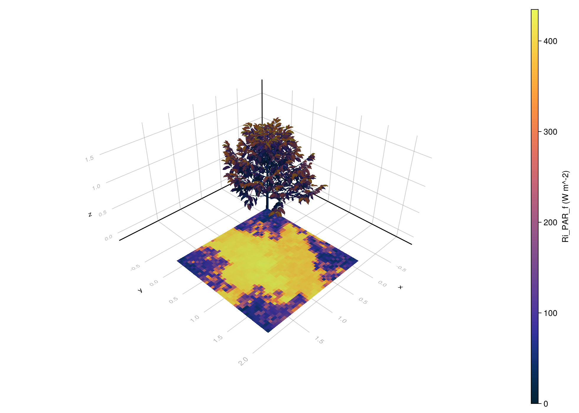

If you do not want to reattach values onto the MTG just for visualization, ArchimedLight.jl also provides a helper that plots directly from the LightStepResult (this is more performant):

fig2, ax2, p2 = lightplot(
    step;
    color=:incident_par_flux,
    colormap=:thermal,
)

Colorbar(fig2[1, 2], p2.plots[1], label="Ri_PAR_f (W m^-2)")
fig2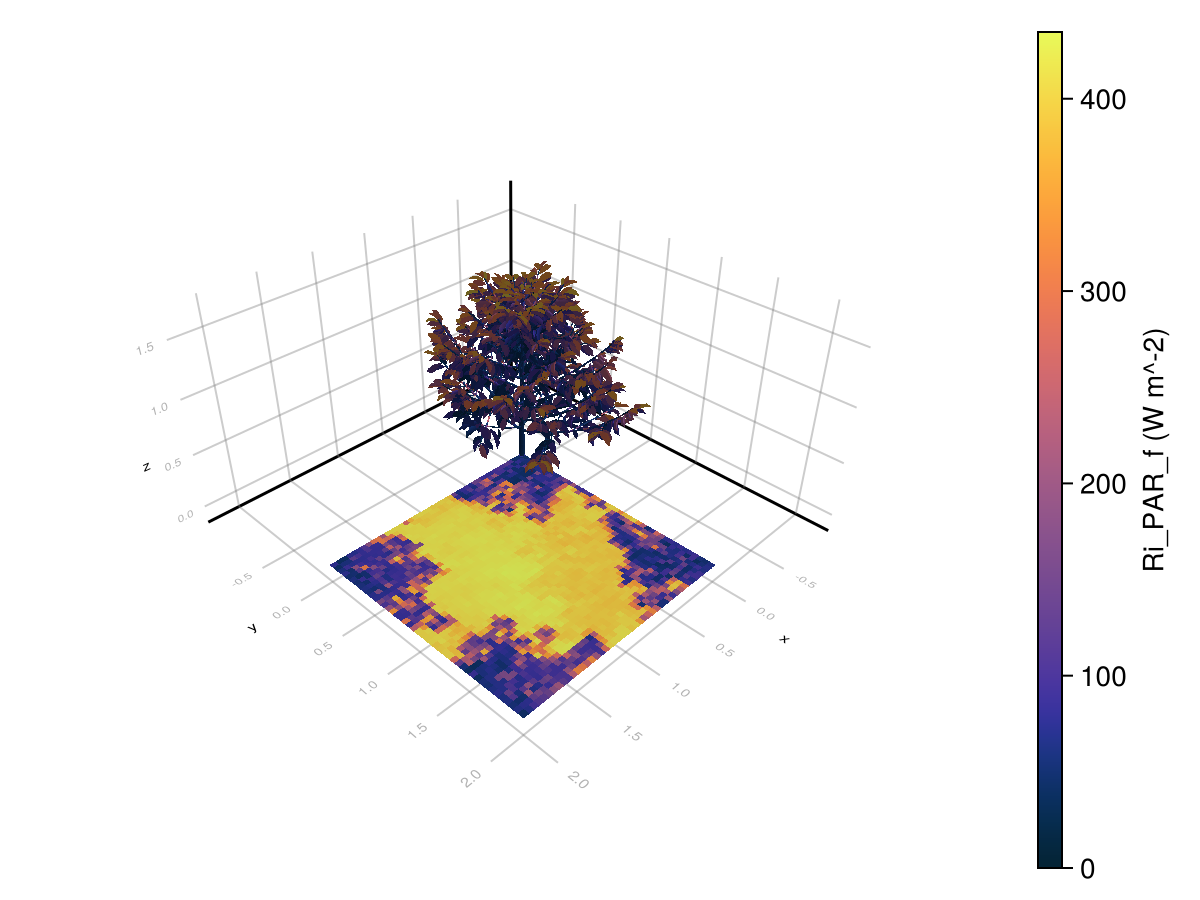

If you want to visualize the same toric result as a repeated tile, build a tiled render geometry from the scene plot bounds and reuse the same light result:

tiled = tile_light_geometry(scene, step; nx=3, ny=3)
fig_inf, ax_inf, p_inf = lightplot(tiled, step; color=:incident_par_flux)
Colorbar(fig_inf[1, 2], p_inf.plots[1], label="Ri_PAR_f (W m^-2)")
fig_inf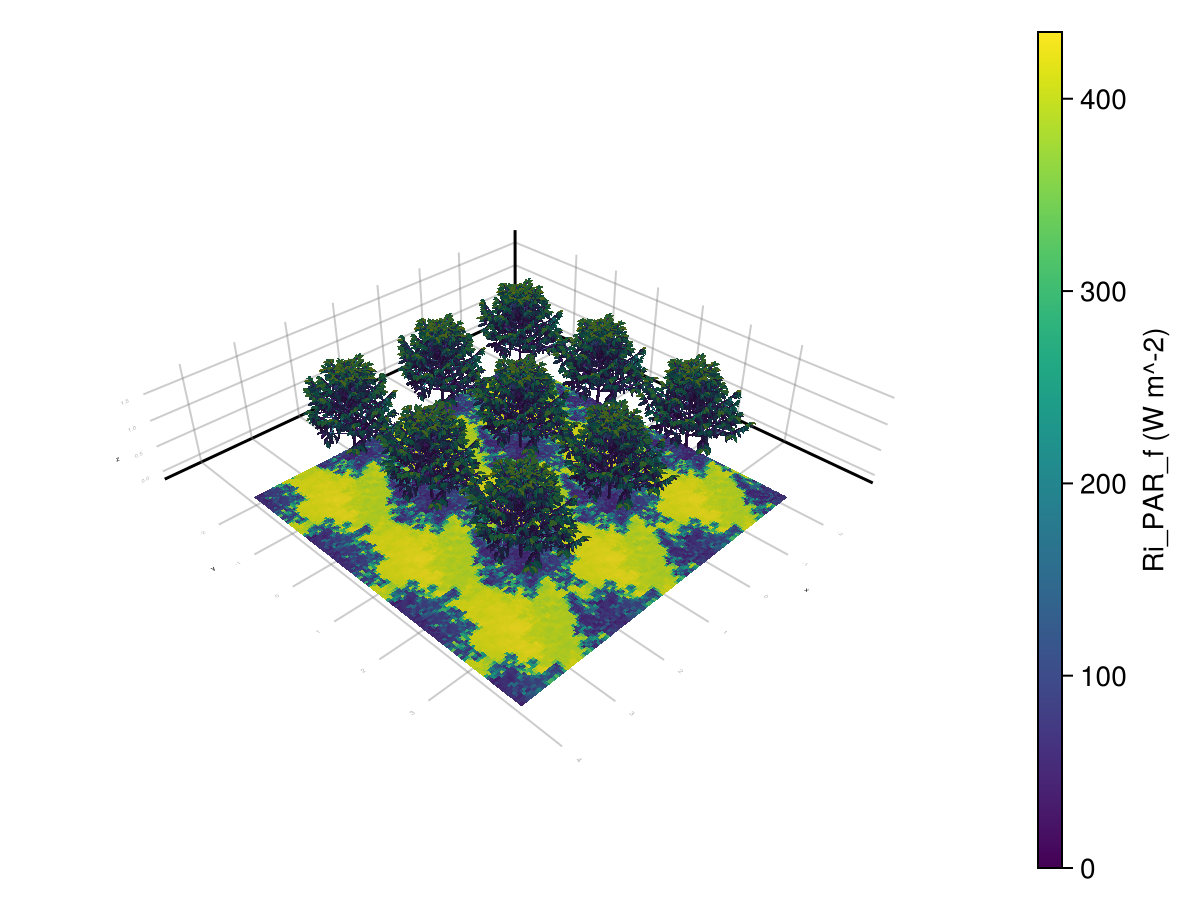

For a time series, we can generate the plot once and update timestep to inspect any simulated hour. Each LightStepResult supplies its own stored render geometry, so this also works for a series assembled from scenes that changed between simulation steps:

# Generating a series of meteo row to simulate a day:
meteo = PlantMeteo.TimeStepTable(
    [
        (
            date=Date(2020, 6, 21),
            hour_start=Time("06:00:00") + Hour(i-1),
            duration=Hour(1),
            latitude=15.0,
            clearness=0.6,
        )
    for i in 1:10],
    (latitude=15.0, file="interactive",),
)

update_options!(sim, LightOptions(turtle_sectors=16, all_in_turtle=true, radiation_timestep_minutes=5, pixel_size=0.003, toricity=true))
series = run_light(sim, meteo)

fig = Figure(resolution=(980, 700))
ax = Axis3(fig[1, 1], title="Intercepted PAR flux over time (06:00)", azimuth=π/4, elevation = π/6, aspect=:data, perspectiveness= 0.4)
p = lightplot!(ax, series; color=:Ri_PAR_f, colormap=:thermal)
Colorbar(fig[1, 2], p.plots[1], label="Ri_PAR_f (W m^-2)")

p[:timestep][] = length(series)
ax.title[] = "Intercepted PAR flux over time ($(Time("06:00") + Hour(length(series)-1)))"
fig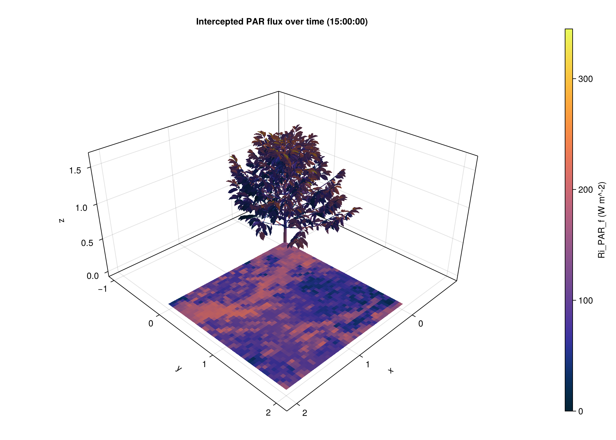

When colorrange is left automatic on a series plot, lightplot(series) uses one color scale for the whole series so the same value maps to the same color at every timestep.

The toricity parameter is activated here, this is why we see the shade of the coffee plant coming from all corners, because light that goes out of the scene on one side comes back in on the other side. This is done for simulating an infinite canopy, but it can be turned off with toricity=false in the config.

One Important Difference From The Historical Java App