Configuration And Options Reference

This page documents the top-level config.yml structure and the light options that the current Julia package actually reads.

The main source of confusion with historical ARCHIMED YAML files is that not all parameters play the same role. Some keys simply point to input files, some control the numerical approximation used by the light algorithm, some switch physical processes on or off, and some exist mainly for parity, debugging, or cache behavior. That is why a good explanation of a parameter cannot stop at "this is a Boolean" or "this is an integer": users need to know what assumption sits behind it and what part of the pipeline will actually read it.

The right mental model is that config.yml is mostly a wiring layer. It connects a scene file, one or more model files, and a meteo file, then adds a set of global runtime options. The scene structure itself lives in .ops / .opf / .gwa, optical properties live in the model YAML files, and time-varying forcing lives in meteo.csv. In practice, most questions about configuration are really questions about how those runtime options affect the light computation once the inputs have been loaded.

Top-Level Keys

The read_simulation(path) entry point reads these top-level keys directly:

scene: scene/coffee.ops
models:
  - models/plant_coffee.yml
  - models/soil.yml
meteo: meteo.csv

sky_sectors: 16
all_in_turtle: false
radiation_timestep: 15
radiation_input_semantics: interval_mean
scene_rotation: 0
scattering: true
pixel_size: 1
area_ratio: true
toricity: true
cache_pixel_table: false
pixel_hit_stack_mode: auto
cache_radiation: false
store_node_metadata: true
node_metadata_attributes: []
check_meteo_boundaries: true
allow_overlapping_meteo_steps: false
scattering_max_iter: 20
scattering_stop_ratio: 0.01
scattering_coeff_par: 0.15
scattering_coeff_nir: 0.30
nir_interception: true
nir_scattering: true
java_logged_turtle_dirs: false
meteo_range: 2, 3
debug: false
log_debug: false
debug_drop_leading_hit:
  node_id: 12
  x: 40
  y: 18

component_variables:
  sky_fraction: false

Required Keys

• scene: path to an .ops, .opf, or .gwa scene source
• models: list of model YAML files, or a config file that itself contains such a list
• meteo: path to the meteo CSV

Without those three keys, read_simulation cannot assemble the simulation inputs.

Where Options Enter The Algorithm

The runtime pipeline is still simple at a high level:

read_simulation
  -> run_light
  -> compute_sky
  -> build_turtle
  -> compute_directional_fluxes
  -> compute_first_order
  -> compute_scattering
  -> integrate_light

What matters is that the options do not all act at the same stage. meteo_range is applied early, when the meteo table is filtered before the series is run. check_meteo_boundaries validates the selected forcing values, while allow_overlapping_meteo_steps decides whether overlapping intervals are rejected or kept. radiation_timestep comes into play when one meteo row is internally subdivided so that the sun path and the direct/diffuse split can be integrated more faithfully. radiation_input_semantics determines how supplied irradiance is converted to a full-step mean, while scene_rotation maps the geographic sun into the scene-local directional basis. sky_sectors, all_in_turtle, and java_logged_turtle_dirs define the directional representation of the sky itself. pixel_size, toricity, area_ratio, cache_pixel_table, pixel_hit_stack_mode, and debug_drop_leading_hit all belong to the raster projection machinery used for first-order interception. The scattering options act later, when intercepted light is propagated iteratively through the canopy. cache_radiation matters only in series mode when directional responses can be reused across many timesteps. store_node_metadata controls the lightweight per-scene metadata snapshot referenced by results, while node_metadata_attributes opts additional scalar MTG identifiers into that snapshot. Requesting sky_fraction in the output variables controls whether an extra per-node sky-view output is stored in each LightStepResult.

This distinction is important for interpretation. Changing pixel_size or sky_sectors does not mean you have changed the plant or the atmosphere; it means you have changed the numerical approximation used to represent them. By contrast, changing scattering, nir_interception, or nir_scattering changes which physical processes are included in the simulation.

Option Reference

sky_sectors

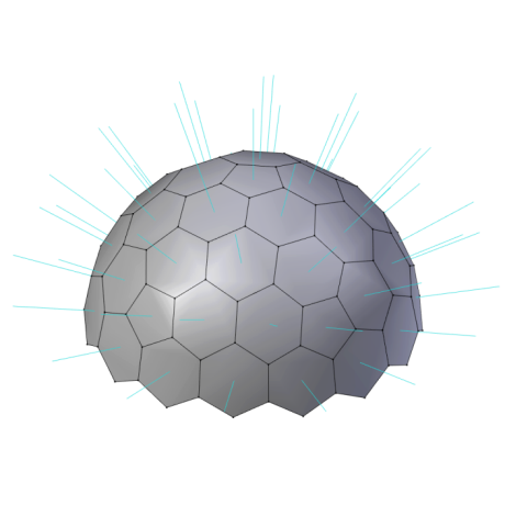
Number of turtle sectors used to discretize the sky hemisphere. Common historical ARCHIMED counts are:

• 1
• 6
• 16
• 46
• 136
• 406

Those values use the ARCHIMED/Java-style turtle construction. Other positive counts are still accepted by the Julia runtime, but they fall back to a generic hemisphere discretization rather than the historical turtle.

This parameter is really the statement that the diffuse sky will not be treated as a continuum. Instead, the hemisphere is replaced by a finite set of incoming directions, and the solver computes interception and scattering sector by sector on that discrete representation. In other words, sky_sectors controls the angular resolution of the light field rather than the scene itself.

In practice, increasing the number of sectors gives a finer directional description of light, which is especially useful when the sky is anisotropic or when canopy structure creates strong directional effects. The tradeoff is straightforward: more sectors mean more directional projections and therefore more computation. So this option changes the numerical approximation of the sky, not the underlying biology or optical properties.

all_in_turtle

Controls how direct light is represented:

• false: keep the direct beam as its own explicit sun direction
• true: redistribute direct light into turtle sectors near the sun direction

This option controls how the direct beam is represented. With false, the sun remains an explicit direction of its own, separate from the diffuse sky sectors. With true, direct irradiance is redistributed into the turtle itself, so that all incoming light is represented on the same directional discretization.

The difference is mostly conceptual and numerical. Keeping the sun explicit is usually clearer because the direct beam remains identifiable as a distinct source, which makes the result easier to reason about. Folding it into the turtle is mainly useful for compatibility with historical ARCHIMED behavior and for workflows that want a single directional basis. The practical effect is that true smooths the direct component angularly, while false preserves it as a separate beam.

radiation_timestep

Maximum duration, in minutes, of the radiative substeps used inside a meteo interval. This is one of the key ARCHIMED ideas: the meteo time step and the radiative integration substep are not the same thing.

If a meteo row spans 30 minutes and radiation_timestep: 5, the direct beam and sky decomposition are evaluated on smaller substeps and integrated back into one directional forcing state. In other words, a meteo row may cover a fairly long interval, but the sun position and the direct/diffuse partition can still change significantly inside that interval. radiation_timestep tells the solver how finely it should subdivide the meteo row before averaging those directional fluxes back together.

Smaller values therefore improve temporal fidelity, especially near sunrise, sunset, or whenever direct light changes rapidly, while larger values are cheaper but coarser.

radiation_input_semantics

Controls what a supplied RI_SW_f, RI_PAR_f, RI_NIR_f, or other shortwave RI_*_f value means when a meteo interval overlaps sunrise or sunset. Accepted values are:

• interval_mean (the default): the supplied value is already the mean over the complete meteo interval. Its full-timestep energy is preserved. During a partly sunlit step, the internally evaluated daylight substeps are scaled so that averaging them over the full interval recovers the supplied value.
• sunlit_intensity: the supplied value applies only during the daylight portion of the interval. This reproduces the historical Java clipping. If daylight lasts for a fraction f of the full step, the effective irradiance is f times the supplied value; a fully nighttime step has zero solar flux.

For example, a two-hour step containing one hour of daylight with RI_PAR_f: 200 produces an effective full-step PAR irradiance of 200 W m^-2 under interval_mean, and 100 W m^-2 under sunlit_intensity. The SkyState returned by compute_sky stores this effective full-step mean, and the directional turtle fluxes sum to the same value without a later energy renormalization.

Choose interval_mean for conventional meteorological tables whose radiation columns are interval means. Choose sunlit_intensity when reproducing Java ARCHIMED results or when the supplied values explicitly describe only the sunlit part of each interval.

If interval-mean input explicitly contains a direct component but its supplied or representative sun lies below the modeled upper hemisphere, there is no physical sun sector to receive that component. ArchimedLight then distributes the otherwise unrepresentable direct share over the available turtle sectors; this conservative fallback preserves the supplied full-step energy.

scene_rotation

Rotation in degrees between geographic north and the scene's local coordinate system. Positive values rotate the geographic sun clockwise into local plot coordinates, matching ARCHIMED's compass-angle convention.

The diffuse turtle sectors themselves remain fixed in the scene-local basis. Only the geographic sun is transformed; clear-sky brightness and direct-beam weights are then evaluated against that transformed sun. This keeps the projection directions and local artificial-emitter quadrature stable while correctly changing which local directions receive anisotropic sky and direct radiation. The equivalent Julia constructor keyword is LightOptions(scene_rotation_deg=...).

pixel_size

Requested pixel size in centimetres in the YAML file. Internally, LightOptions.pixel_size stores the value in meters.

This parameter controls the horizontal sampling density of the projected pixel tables:

• smaller pixels -> more rays and finer spatial resolution
• larger pixels -> fewer rays and faster runs

The current runtime validates 0 < pixel_size <= 0.5 meters after conversion.

This parameter is one of the main numerical controls in the whole model because first-order interception is computed by rasterizing projected geometry onto a regular horizontal grid. pixel_size therefore sets the spatial resolution of that projection.

Smaller pixels produce a finer approximation of canopy geometry. They resolve small gaps better, distinguish nearby components more clearly, and generally reduce discretization artefacts, but they also increase the number of pixels and the size of the hit tables the solver has to manage. Larger pixels make runs cheaper, but they can merge nearby organs into the same projected cell and smooth out the structure of the canopy.

area_ratio

Whether to apply the projected-area correction after rasterization. For ARCHIMED-style parity, this normally stays enabled.

See First-Order Interception for the geometric reason this correction exists.

The point of area_ratio is to acknowledge that the area covered by hit pixels is only an approximation of the true projected mesh area. After rasterization, the solver can compare those two quantities and use their ratio as a correction factor. When area_ratio is enabled, this correction is applied node by node; when it is disabled, the raw rasterized area is used as-is.

In practice, leaving this on usually makes the result less sensitive to pixelization artefacts and more consistent with the underlying geometry, which is why it is the normal setting for ARCHIMED-style parity. Turning it off is mainly useful if you explicitly want to inspect the uncorrected raster behavior or reproduce a simplified approximation.

scattering

Enable or disable iterative multiple scattering.

• false: first-order interception only
• true: first-order interception followed by iterative scattering

This option controls whether the model stops after first-order interception or continues with iterative multiple scattering. With scattering disabled, the simulation only answers the question "what does the incoming light hit first?" With scattering enabled, intercepted light can be reflected or re-emitted and can illuminate other components again, possibly over several iterations.

That makes scattering a physical-process switch, not just a performance setting. Turning it off is faster and often easier to interpret, but it removes an important redistribution mechanism in dense canopies and in wavebands such as NIR where scattering is typically stronger. Turning it on adds cost, but it makes the simulation closer to the full ARCHIMED light balance.

scattering_max_iter

Hard cap on the number of scattering iterations.

The scattering stage is solved iteratively rather than in one closed-form step, so the model needs a stopping rule. scattering_max_iter is the hard ceiling: even if the solver has not yet decayed below its stopping threshold, it will stop once this number of iterations has been reached.

Conceptually, increasing the cap lets the model retain more late and weak scattering exchanges. In many cases nothing changes, because the solution has already stabilized before the cap is reached. But if a scene is highly scattering or the stopping tolerance is strict, this parameter can become active and then it directly controls how far the propagation is allowed to continue.

scattering_stop_ratio

Relative stopping threshold for scattering. The iterative process stops when the scene-scale scattered energy of the current iteration falls below:

scattering_stop_ratio × initial intercepted scene energy

The default 0.01 reproduces the historical 1 percent rule.

This is the soft stopping rule for the same iterative solver. The idea is that later scattering iterations eventually become weak enough to be negligible compared with the initially intercepted energy. The solver therefore computes a threshold from the initial scene-scale intercepted energy and stops when the energy carried by the current scattering iteration falls below scattering_stop_ratio times that reference value.

In practical terms, this is the main accuracy-versus-speed knob inside the scattering stage. Smaller values keep weaker late iterations and therefore run longer, while larger values stop earlier and may truncate the long tail of scattering contributions. The default 0.01 is there to reproduce the historical 1 percent ARCHIMED rule.

scattering_coeff_par, scattering_coeff_nir

Fallback scattering coefficients used when the relevant model file does not provide optical_properties for the corresponding waveband.

The current defaults are:

• PAR: 0.15
• NIR: 0.30

Absorptance is derived as 1 - scattering_coefficient unless more specific per-node information is available.

These parameters are fallbacks, not the preferred place to describe optics. If a model file already provides waveband-specific optical properties, those values are used. But if some components have no explicit optical description, the solver still needs default coefficients telling it what fraction of intercepted energy remains available for scattering in PAR and in NIR.

That is why these coefficients matter in two ways at once. They determine how much energy is re-injected into the canopy during the scattering stage, and they also imply a default absorptance of 1 - coefficient during budget integration. In practice, the PAR and NIR values should usually not be the same, because plant tissues are typically much more scattering in NIR than in PAR. These settings are therefore best understood as safety nets for incomplete model files, not as the main calibration interface.

cache_radiation

Reuse directional light responses across meteo rows. This is worthwhile when many time steps are simulated on the same scene.

cache_radiation exists because, for a fixed scene and a fixed directional discretization, the expensive part of the first-order computation is often the directional response itself rather than the meteo-dependent weighting of those responses. In a time series, many rows may reuse the same turtle structure and the same geometric projections, so it is wasteful to rebuild them every time.

When this option is enabled, run_light(sim, meteo) and repeated run_light(sim, row) calls reuse unit directional responses across meteo rows. In the raster CPU path, that cache stores the first-order response and, when scattering is enabled, the scattered added-light response as well. The time-step results are then reconstructed by weighting those cached unit responses with the true directional fluxes of each row.

The main effect is therefore still on runtime, not on physics, but the optimization is now stronger than a simple first-order shortcut. It is especially useful for long series on an unchanged scene and for manual simulation loops where you run a few steps, pause, inspect or grow the scene, and then explicitly rebuild the cache when geometry or optics change.

Large scenes are handled with a tiered policy. If the full-response cache is small enough, it stays in memory. If not, the runtime falls back to a bounded partial cache, and if even that is not appropriate it falls back to the prepared topology path instead of allocating an unbounded cache.

sky_fraction output request

Store a per-node sky_fraction dictionary in each LightStepResult by asking for the historical output variable:

component_variables:
  sky_fraction: true

The same applies if sky_fraction: true appears in opf_variables, including when opf_variables reuses the same YAML anchor as component_variables.

This output is useful for coupled models such as PlantBiophysics that need a sky-view fraction on each MTG object. When requested, read_options sets LightOptions.include_sky_fraction=true, and attach_light_step! / attach_light_series! can export it back to the MTG with fields=[:sky_fraction].

The calculation reuses the same directional visible-area machinery as the light interception code. Because it is an additional output and not needed for the core light budget, it is not stored unless the output variable is requested or LightOptions(include_sky_fraction=true) is constructed directly in Julia.

cache_pixel_table

Store projection tables on disk instead of recomputing or keeping them only in memory. This trades recomputation for disk I/O.

Where cache_radiation works at the series level, cache_pixel_table works one layer lower, inside the raster projection machinery. The idea is that if the scene geometry, direction, toricity, and projection grid are unchanged, the corresponding pixel table can be serialized and reused instead of being recomputed from scratch.

This option should not change the physical result. Its role is purely practical: it can save time in repeated runs of the same scene and configuration, especially in parity work or when rebuilding documentation examples. It becomes much less useful once geometry or numerical options are changing frequently, because those changes invalidate the cache key and force a rebuild anyway.

toricity

Enable the periodic wrapping of the plot in the horizontal plane.

• false: the plot is treated as isolated
• true: rays leaving one horizontal edge re-enter on the opposite edge

This is how ARCHIMED represents repeated orchard or crop patterns with a finite representative tile.

When it is enabled, the plot is treated as one tile of an infinite periodic repetition in the horizontal plane. Rays leaving one side of the plot re-enter from the opposite side, so the canopy no longer has true horizontal borders in the radiative sense.

That can be very appropriate for repeated crop rows or orchard motifs, because it removes edge effects that would otherwise be artefacts of simulating only one finite tile. But it would be the wrong choice for an isolated plant or a genuinely finite experimental plot, because then those edge losses are part of the situation being modeled. In other words, toricity changes the geometry that the solver "sees", not merely the efficiency of the calculation.

For reference, we call this option "toricity" because it effectively turns the horizontal plane into a torus. The vertical dimension remains unchanged, so the plot is still finite in height, but the horizontal plane wraps around on itself like a donut:

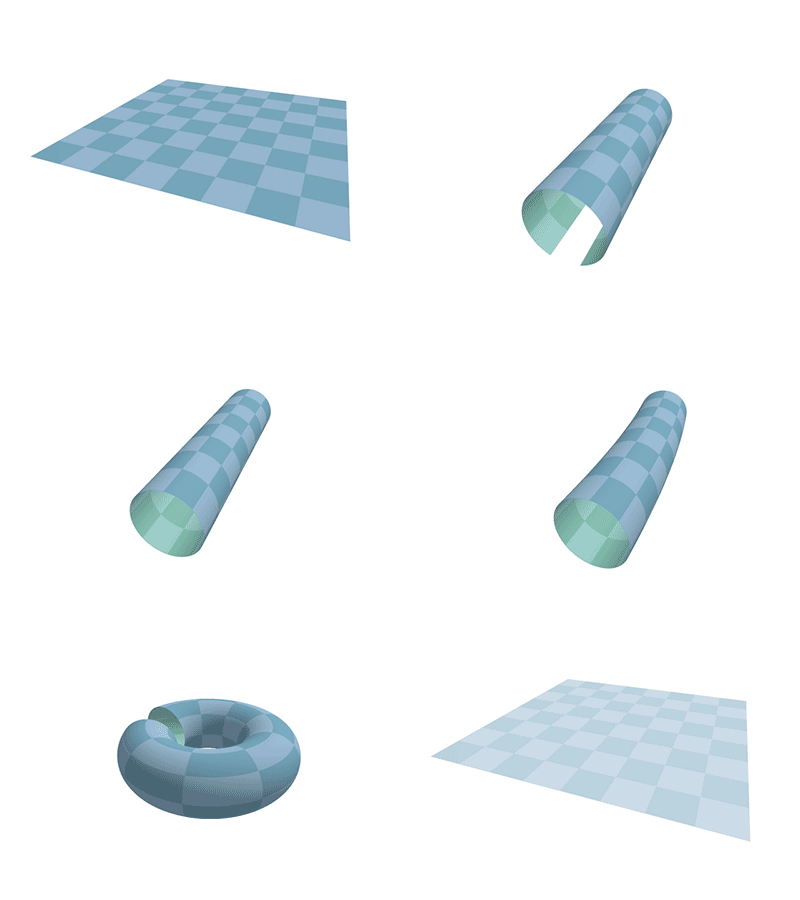
So if you simulate a scene with toricity: true and then visualize the result, you should see projected shadow patterns across the horizontal edges, as if the plot were repeated infinitely in all horizontal directions. For example, the coffee scene with toricity enabled looks like this:

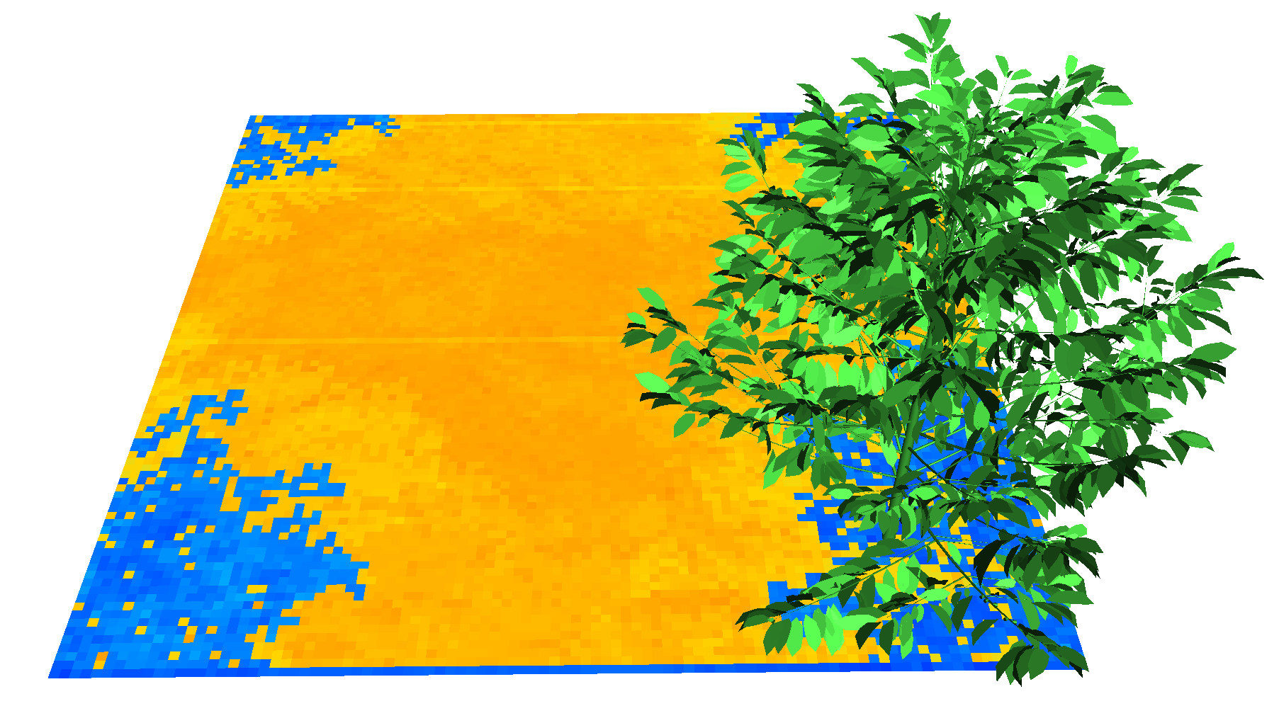
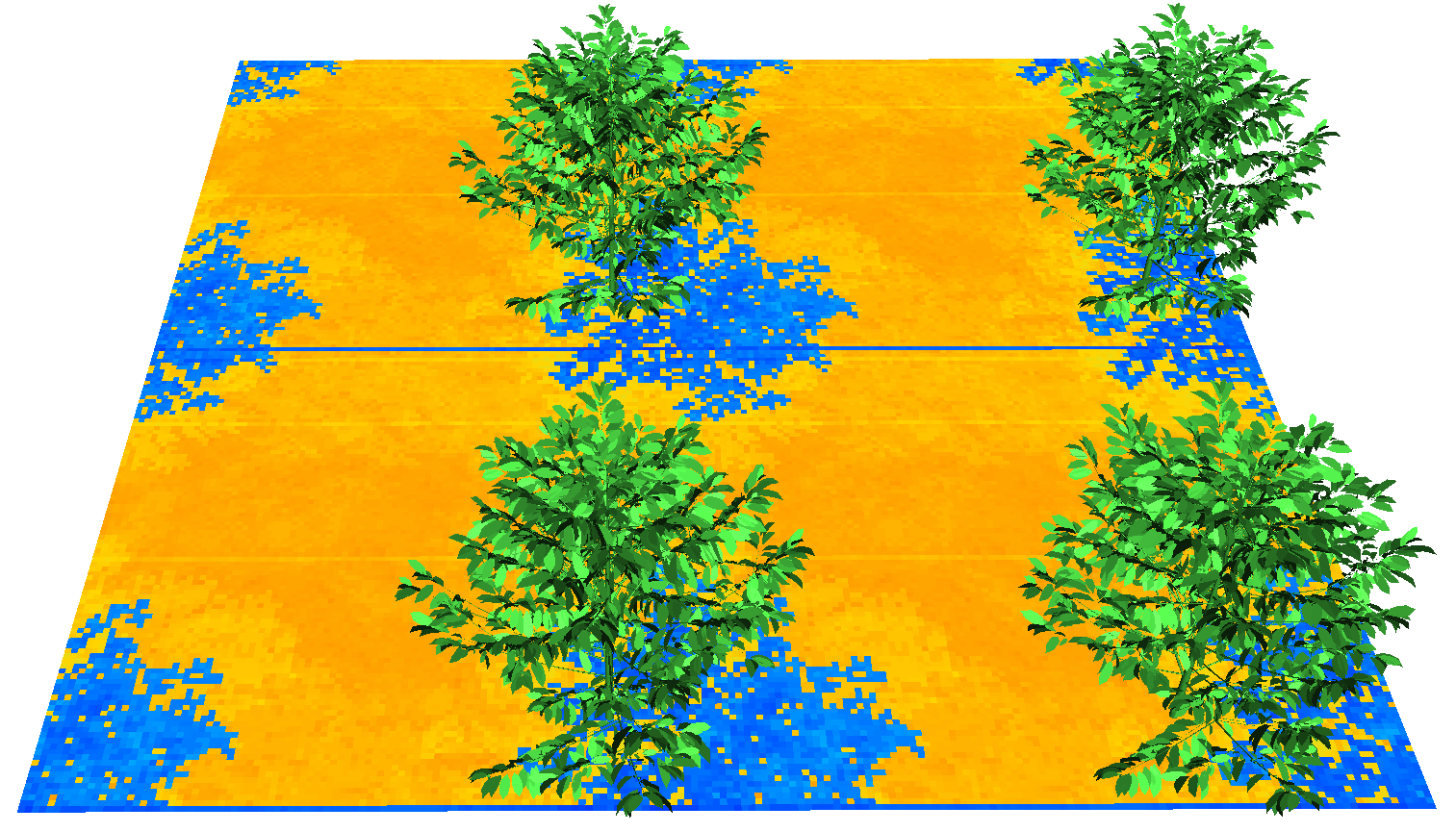
We can see that there is a shadow on the ground, on all corners, because the coffee plant is put on the bottom-right corner of the plot and therefore casts a shadow that wraps around the horizontal edges. The same toric result repeated for visualization looks like this:

nir_interception, nir_scattering

Allow you to disable NIR interception or NIR scattering independently when needed for debugging, parity work, or reduced runs.

These options exist because the runtime carries PAR and NIR as separate wavebands, and some studies or debugging workflows may want to simplify the calculation. nir_interception is the broader switch: if it is disabled, NIR is removed before the directional fluxes and interception stages, so there is effectively no NIR light in the run. This includes NIR from artificial emitters, both received and escaped. nir_scattering is narrower: it keeps the first-order NIR interception but skips the NIR multiple-scattering stage.

For normal scientific runs, these options are usually left enabled. Turning them off is mainly useful for parity work, reduced experiments, or targeted diagnostics. The distinction matters because nir_scattering: false still retains a first-order NIR contribution, whereas nir_interception: false removes the NIR branch much earlier and therefore changes the energy budget more strongly.

java_logged_turtle_dirs

Compatibility/debug option for Java-style turtle direction logging.

This parameter is there for parity rather than for modeling. In principle, two turtle constructions can be mathematically "the same" while still differing slightly because of ordering, logging history, or Float32-level implementation details. Those small differences matter when the goal is to reproduce historical Java results as closely as possible.

When java_logged_turtle_dirs is enabled, build_turtle uses the compatibility path based on Java-style directions. That can be useful during fixture matching or debugging old workflows, but it should not be treated as a scientific calibration parameter. For ordinary use, the default behavior is usually the right choice.

meteo_range

Restrict the simulated meteo rows. The historical string forms are still accepted, for example:

meteo_range: 2, 5
# or
meteo_range: 2016/07/01 08:00:00, 2016/07/01 12:00:00

meteo_range simply helps select the meteo rows. That makes it useful whenever a full meteo file contains more data than the run you are trying to reproduce, inspect, or debug.

The range is applied during prepare_meteo, after the sequence has been validated, and it can be expressed either with row indices or with datetimes. After that, the optional active field in the meteo table can still remove rows one by one.

check_meteo_boundaries

Enable physical range checks for the selected meteorological forcing. The default is true. It rejects negative irradiance, clearness or direct fractions outside [0, 1], invalid latitude and sun-angle ranges, and nonpositive durations before numerical work begins.

Set this to false only for a deliberate research or compatibility input:

check_meteo_boundaries: false

This disables range checks only. ArchimedLight still requires a positive duration, a derivable radiation and solar-geometry path, and consistency among redundant finite inputs. In Julia, a one-call override is also available as run_light(sim, meteo; check_boundaries=false).

allow_overlapping_meteo_steps

Allow overlapping meteo intervals to pass through prepare_meteo and run_light_series.

allow_overlapping_meteo_steps: true

By default the Julia runtime rejects series where one meteo step starts before the previous one ends. That is usually the right default because it catches inconsistent forcing tables early. But some historical workflows intentionally reuse partially overlapping meteo intervals, for example when several forcing windows describe the same day with different aggregation choices.

When this flag is true, that validation is skipped and the rows are kept in their original order. The light solver then treats each row independently. This option only changes the preparation-time consistency check; it does not merge rows, resolve overlaps, or change how one row is integrated internally.

pixel_hit_stack_mode

Internal raster-storage option controlling how per-pixel hit stacks are stored. Supported values are:

• auto
• small
• vector

This option is purely about implementation strategy inside the raster code. It selects how per-pixel hit stacks are stored in memory, which can matter for performance or for low-level debugging, but it is not intended to represent any physical assumption.

For most users, auto is the correct setting and should be left alone. The other modes are mainly there when you are investigating performance behavior or trying to isolate an implementation-level discrepancy in the interception code. They are not meant to change the semantics of the model.

debug, log_debug, debug_drop_leading_hit

Low-level parity and debugging options used mainly while chasing differences with the Java implementation.

These parameters are not part of the scientific interface. They are instrumentation and fault-injection controls used when chasing low-level mismatches, especially against the Java implementation. debug and log_debug enable extra tracing, while debug_drop_leading_hit goes further and deliberately removes the leading hit from one chosen pixel stack when a very specific condition is met.

That last option is intentionally invasive: it changes the interception result in one localized place so that a mismatch can be isolated and understood. For that reason, all of these options should be thought of as developer tools, not user-facing model parameters. Outside parity investigations, they should remain disabled.

Legacy Keys You May Still See

The bundled examples intentionally preserve several historical ARCHIMED keys such as:

• photosynthesis
• output_directory
• simulation_directory
• write_summary
• export_ops
• component_variables
• opf_variables

Those keys remain useful documentation for old workflows, but they are not the main user API of the current light-only Julia package. One exception is sky_fraction: requesting it in component_variables or opf_variables is honored so the value is available for later attachment. For actual output pathways in ArchimedLight.jl, see Outputs.

Recommended Reading Order

• Scene Files And Semantics
• Model Files Reference
• Meteo Inputs Reference

Interactive Equivalent

The config.yml file is convenient if you want to store the configuration on portable files that you can also reuse with the historical java implementation. However, if you are working interactively in Julia, you can pass the same information directly to LightSimulation by instantiating a LightOptions struct and building the scene, models, and meteo in memory:

options = LightOptions()
sim = LightSimulation(scene, models; options=options)
step = run_light(sim, first(rows))

For example, this file-based block:

sky_sectors: 16
pixel_size: 1
toricity: true
scattering: false

becomes:

options = LightOptions(
    turtle_sectors=16,
    pixel_size=0.01, # Note that pixel_size is in meters in the Julia API
    toricity=true,
    scattering=false,
)

The parameters are the same, you can see the full list in the documentation for LightOptions.