Outputs

The current Julia package exposes light results in three increasingly concrete forms:

1. in memory as LightBudget
2. attached back onto MTG nodes as ARCHIMED-style attributes
3. written to disk when you export the enriched scene

This page documents those three layers and then explains the ARCHIMED-style CSV outputs used by the public writer and regression harness.

1. In-Memory Outputs: LightBudget

The core output of run_light for one meteo row is:

using ArchimedLight

repo_root = normpath(joinpath(dirname(pathof(ArchimedLight)), ".."))
config = joinpath(repo_root, "example_2", "config.yml")
sim, meteo = read_simulation(config)
sky_options = LightOptions(sim.options; include_sky_fraction=true)
sim = LightSimulation(sim.scene, sim.models; options=sky_options)
row = first(meteo)
step = run_light(sim, row)
budget = step.budget;

LightBudget(ArchimedLight.InitialTotalSpectralNodeValues(ArchimedLight.SpectralNodeValues(Dict(3988 => 289.90128719635203, 601 => 176.0083256429957, 1356 => 65.3655161967034, 4651 => 354.1097378808897, 3233 => 268.81355554181255, 960 => 142.0911613802784, 2874 => 115.15725927789562, 205 => 204.8795666747116, 5010 => 360.8821544834643, 5406 => 419.8532862204779…), Dict(3988 => 314.059727796048, 601 => 190.67568611324538, 1356 => 70.81264254642868, 4651 => 383.6188827042972, 3233 => 291.21468517029695, 960 => 153.93209149530165, 2874 => 124.75369755105359, 205 => 221.9528638976043, 5010 => 390.95566735708627, 5406 => 454.8410600721845…)), ArchimedLight.SpectralNodeValues(Dict(3988 => 320.1587097672037, 601 => 200.0689224622859, 1356 => 85.03103241867859, 4651 => 359.4487855968359, 3233 => 293.22199731164545, 960 => 172.31615855455922, 2874 => 134.16282851481844, 205 => 232.28467700608698, 5010 => 364.2503137185889, 5406 => 424.053871137096…), Dict(3988 => 707.1442907655063, 601 => 661.1552489318191, 1356 => 447.2246568590664, 4651 => 504.0757473814203, 3233 => 648.4795934521438, 960 => 638.9699033284262, 2874 => 494.45313129959527, 205 => 673.8565187449592, 5010 => 480.7391917008195, 5406 => 564.0019826746656…))), ArchimedLight.InitialTotalSpectralNodeValues(ArchimedLight.SpectralNodeValues(Dict(3988 => 93.26936346427601, 601 => 26.406534400384555, 1356 => 347.91735865920487, 4651 => 1316.9371202012123, 3233 => 2287.5958138171623, 960 => 757.6982664100082, 2874 => 612.941075673925, 205 => 1244.464641192095, 5010 => 1342.1229150526178, 5406 => 1561.434863110915…), Dict(3988 => 101.04181041963234, 601 => 28.60707893374994, 1356 => 376.9104718808053, 4651 => 1426.6818802179803, 3233 => 2478.2287983019255, 960 => 820.8397886108424, 2874 => 664.0194986467521, 205 => 1348.1700279581032, 5010 => 1453.9664913070023, 5406 => 1691.5544350368252…)), ArchimedLight.SpectralNodeValues(Dict(3988 => 103.00402373621034, 601 => 30.01634646626994, 1356 => 452.5898963934731, 4651 => 1336.793083964683, 3233 => 2495.310968292639, 960 => 918.8724572515406, 2874 => 714.1009515247633, 205 => 1410.9267796517738, 5010 => 1354.6491196178645, 5406 => 1577.0568433347905…), Dict(3988 => 227.50812359251103, 601 => 99.19314192173654, 1356 => 2380.4175411609913, 4651 => 1874.6619821651248, 3233 => 5518.543141684069, 960 => 3407.2941859092743, 2874 => 2631.797908959862, 205 => 4093.0905137374425, 5010 => 1787.8719613305423, 5406 => 2097.5240340251703…))), ArchimedLight.InitialTotalSpectralNodeValues(ArchimedLight.SpectralNodeValues(Dict(3988 => 246.41609411689922, 601 => 149.60707679654632, 1356 => 55.56068876719789, 4651 => 300.99327719875623, 3233 => 228.49152221054067, 960 => 120.77748717323664, 2874 => 97.88367038621128, 205 => 174.14763167350486, 5010 => 306.74983131094467, 5406 => 356.87529328740624…), Dict(3988 => 31.40597277960479, 601 => 19.067568611324532, 1356 => 7.081264254642866, 4651 => 38.361888270429716, 3233 => 29.121468517029687, 960 => 15.393209149530161, 2874 => 12.475369755105357, 205 => 22.195286389760422, 5010 => 39.095566735708616, 5406 => 45.48410600721844…)), ArchimedLight.SpectralNodeValues(Dict(3988 => 272.1349033021231, 601 => 170.05858409294302, 1356 => 72.2763775558768, 4651 => 305.5314677573105, 3233 => 249.23869771489862, 960 => 146.46873477137532, 2874 => 114.03840423759567, 205 => 197.44197545517392, 5010 => 309.61276666080056, 5406 => 360.4457904665316…), Dict(3988 => 70.71442907655062, 601 => 66.1155248931819, 1356 => 44.72246568590663, 4651 => 50.40757473814202, 3233 => 64.84795934521436, 960 => 63.896990332842606, 2874 => 49.445313129959516, 205 => 67.3856518744959, 5010 => 48.073919170081936, 5406 => 56.40019826746654…))), ArchimedLight.InitialTotalSpectralNodeValues(ArchimedLight.SpectralNodeValues(Dict(3988 => 79.27895894463461, 601 => 22.44555424032687, 1356 => 295.72975486032414, 4651 => 1119.3965521710306, 3233 => 1944.4564417445877, 960 => 644.0435264485069, 2874 => 520.9999143228362, 205 => 1057.7949450132808, 5010 => 1140.8044777947252, 5406 => 1327.2196336442778…), Dict(3988 => 10.104181041963232, 601 => 2.8607078933749936, 1356 => 37.69104718808052, 4651 => 142.668188021798, 3233 => 247.82287983019253, 960 => 82.08397886108422, 2874 => 66.40194986467519, 205 => 134.8170027958103, 5010 => 145.3966491307002, 5406 => 169.15544350368248…)), ArchimedLight.SpectralNodeValues(Dict(3988 => 87.55342017577878, 601 => 25.51389449632945, 1356 => 384.7014119344521, 4651 => 1136.2741213699805, 3233 => 2121.014323048743, 960 => 781.0415886638094, 2874 => 606.9858087960488, 205 => 1199.2877627040077, 5010 => 1151.4517516751848, 5406 => 1340.4983168345718…), Dict(3988 => 22.750812359251096, 601 => 9.919314192173653, 1356 => 238.04175411609907, 4651 => 187.46619821651245, 3233 => 551.8543141684067, 960 => 340.72941859092737, 2874 => 263.1797908959862, 205 => 409.3090513737441, 5010 => 178.78719613305418, 5406 => 209.75240340251696…))), Dict{String, Dict{Int64, Float64}}(), Dict{String, Dict{Int64, Float64}}(), Dict("PAR" => Dict(), "NIR" => Dict()))

The main grouped fields are:

• budget.incident_flux
• budget.incident_energy
• budget.absorbed_flux
• budget.absorbed_energy

Each one is then split into:

• initial: first-order interception only
• total: first-order plus scattering

and by waveband, for example:

• par
• nir

Typical accesses:

budget.incident_flux.initial.par;
budget.incident_flux.total.par;
budget.absorbed_energy.total.nir;

Dict{Int64, Float64} with 5968 entries:
  3988 => 22.7508
  601  => 9.91931
  1356 => 238.042
  4651 => 187.466
  3233 => 551.854
  960  => 340.729
  2874 => 263.18
  205  => 409.309
  5010 => 178.787
  5406 => 209.752
  2478 => 43.6003
  2082 => 347.211
  5369 => 188.144
  5802 => 213.138
  564  => 46.6726
  2837 => 33.0001
  4255 => 143.358
  3629 => 36.7496
  3196 => 70.5961
  ⋮    => ⋮

Each leaf of that structure is a dictionary keyed by node id.

For artificial emitters, step.first_order.emitter_escaped_power.par and .nir report emitted power which left the represented scene without a geometric hit. These dictionaries are keyed by emitting source node. Together with emitter-contributed incident power, they provide the explicit received-plus-escaped power closure (in W) described in Artificial Light Emitters. Virtual sensors are non-consuming observations: their reported incident power is not subtracted from the ray and is excluded from this physical received-plus-escaped closure. A sensor may therefore report the same ray that is subsequently received by a physical component or escapes the scene. first_order.incident_power combines artificial emitters with sky and sun sources. To verify the closure from public fields, external sky/sun input must be zero and incident power must be summed over physical (non-sensor) receivers; sensor entries are observations, not consumed power. The emitter transfer is accounted separately before it is merged into total incident power. emitter_escaped_power exposes instantaneous PAR and NIR power. The integrated step budget exposes every emitted band, including custom bands, through step.budget.emitter_escaped_energy_per_band[band]. For PAR and NIR this is the corresponding escaped power multiplied by the step duration in seconds.

If you need canopy-view metadata for coupled models, step.sky_fraction stores the per-node visible-sky fraction when options.include_sky_fraction=true. When using a YAML config, read_options enables that option when component_variables.sky_fraction or opf_variables.sky_fraction is true.

2. Query Values By Scene Metadata

light_metric_values combines a light result with its scene metadata and returns a Tables.jl-compatible column table:

coffee_leaves = light_metric_values(
    sim,
    step,
    :absorbed_par_energy;
    species="coffee",
    object_id=1,
    symbol=:Leaf,
)

propertynames(coffee_leaves)

(:step_number, :node_id, :source_topology_id, :object_id, :item_id, :component_id, :group, :type, :symbol, :scale, :value)

The table includes the timestep, runtime and source node identifiers, object and output grouping identifiers, group/type, MTG symbol and scale, and the selected value. A series produces the same columns in long form:

coffee_series = light_metric_values(
    sim,
    [step],
    :Ra_PAR_q;
    species="coffee",
)

unique(coffee_series.step_number)

1-element Vector{Int64}:
 1

All filters combine. group and species are aliases, object_id identifies one placed scene object, source_topology_id identifies its source component, and node_ids accepts one runtime node id or a collection. symbol, scale, type, exact attributes, and a custom where node predicate provide progressively more specific selection.

Selections can be reused:

leaf_ids = light_node_ids(sim; species="coffee", symbol=:Leaf)
leaf_par = light_metric_values(sim, step, :Ra_PAR_q; node_ids=leaf_ids)
leaf_nir = light_metric_values(sim, step, :Ra_NIR_q; node_ids=leaf_ids)
length(leaf_par.value) == length(leaf_nir.value)

true

Use reduce=sum for a total. For example, these compute the whole-scene absorbed PAR and the plant-only total after excluding paving:

scene_absorbed_par = light_metric_values(
    sim,
    step,
    :absorbed_par_energy;
    reduce=sum,
)

plant_ids = setdiff(
    light_node_ids(sim),
    light_node_ids(sim; group="pavement"),
)
plant_absorbed_par = light_metric_values(
    sim,
    step,
    :absorbed_par_energy;
    node_ids=plant_ids,
    reduce=sum,
)

scene_absorbed_par >= plant_absorbed_par

true

Adding by, such as by=:object_id or by=(:group, :type), returns a grouped table. For a series, step_number is retained automatically. sink=DataFrame can materialize detailed or grouped results when DataFrames.jl is loaded.

Summing per-component energy (*_energy or historical *_q) gives an energy total. Flux values are normalized independently by each component's area, so their direct sum generally is not a meaningful scene-scale flux.

Dynamic scenes

Each result retains a lightweight node metadata snapshot by default. All steps computed without changing the scene share the same snapshot. After update_scene!, the next result receives a new snapshot, allowing one series to contain several runtime node-id layouts safely:

steps = LightStepResult[]
for (new_scene, row) in zip(scenes, meteo)
    update_scene!(sim, new_scene)
    push!(steps, run_light(sim, row))
end

second_coffee_leaf = light_metric_values(
    sim,
    steps,
    :absorbed_par_energy;
    species="coffee",
    object_id=2,
    source_topology_id=42,
)

The stable component identity is normally (object_id, source_topology_id); runtime node_id remains local to one scene version. To retain additional scalar identifiers, construct options with node_metadata_attributes=(:organ_id, ...) and filter with attributes=(organ_id=...,). Set store_node_metadata=false when results are queried immediately and minimum retained memory is more important.

3. Attached Outputs: ARCHIMED Attribute Names

The convenience layer for visual inspection is attach_light_step!:

attach_light_step!(
    sim.scene,
    step;
    fields=[:incident_par_flux, :incident_par_energy, :absorbed_par_energy],
);

/ 1: Scene
├─ / 2: Individual
│  └─ / 3: Axis
│     ├─ / 4: Metamer
│     ├─ < 5: Metamer
│     ├─ < 6: Metamer
│     ├─ < 7: Metamer
│     ├─ < 8: Metamer
│     ├─ < 9: Metamer
│     ├─ < 10: Metamer
│     ├─ < 11: Metamer
│     │  ├─ + 12: Axis
│     │  │  ├─ / 13: Metamer
│     │  │  ├─ < 14: Metamer
│     │  │  ├─ < 15: Metamer
│     │  │  ├─ < 16: Metamer
│     │  │  ├─ < 17: Metamer
│     │  │  ├─ < 18: Metamer
│     │  │  ├─ < 19: Metamer
│     │  │  │  └─ + 20: Axis
│     │  │  │     ├─ / 21: Metamer
│     │  │  │     ├─ < 22: Metamer
│     │  │  │     ├─ < 23: Metamer
│     │  │  │     ├─ < 24: Metamer
…

The default mappings are:

The meaning follows the historical ARCHIMED naming:

• area: prepared object surface area in m^2
• Ri: intercepted radiation
• Ra: absorbed radiation
• _0_: first-order only
• no _0_: after scattering has been added
• _f: irradiance-like quantity in W m^-2
• _q: energy per component and per step in J

Shortwave radiation is the sum of its PAR and NIR wavebands. In particular, Ra_SW_f is not an alias for Ra_NIR_f. The typed component and source-owner tables derive it as

\[Ra\_SW\_f = Ra\_PAR\_f + Ra\_NIR\_f.\]

The table also derives aPPFD from absorbed PAR using the requested PAR-energy-to-photon conversion factor:

owner_light = component_values(step; level=:source_owner)
all(isapprox.(
    owner_light.Ra_SW_f,
    owner_light.Ra_PAR_f .+ owner_light.Ra_NIR_f,
))

true

If a downstream package reads attributes attached to the scene, attach the PAR and NIR values under distinct names. Request :absorbed_shortwave_flux to attach their sum as Ra_SW_f. The historical Dict(:absorbed_nir_flux => :Ra_SW_f) mapping remains accepted and now produces the same PAR+NIR sum, with a deprecation warning.

4. Disk Outputs: Exported Scenes

Once results are attached, you can export the enriched scene:

scene_path = joinpath(mktempdir(), "scene_with_light.opf")
write_scene(scene_path, sim.scene)
isfile(scene_path)

true

Supported export formats are:

• .ops
• .opf
• .gwa

The export path determines the format.

This is currently the main disk output mechanism of ArchimedLight.jl: attach node attributes, then write the scene back out.

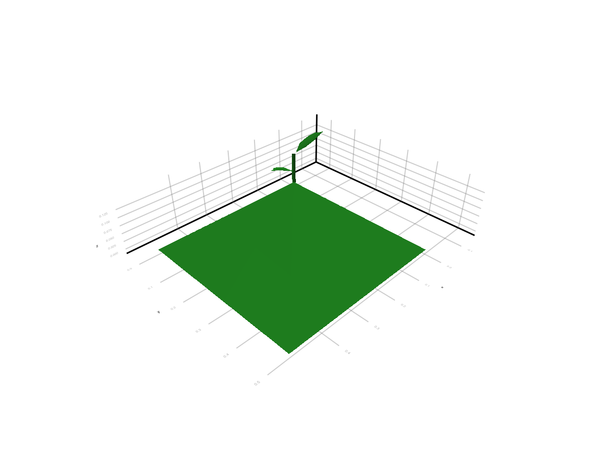
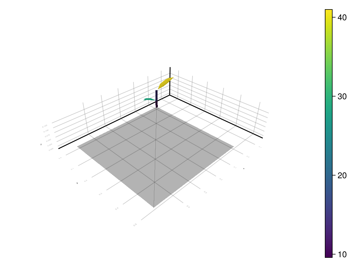
Example Output Images

ARCHIMED-Style CSV Tables

The public writer produces component_values.csv. Historical fixture datasets and internal regression tools may also contain files such as:

• component_values.csv
• scene_values.csv
• summary.csv

The example writes a fresh component_values.csv on demand, while the regression and release harnesses under test/ keep their own isolated reference data.

component_values.csv

Component-scale outputs, typically one row per scene node and step. Common columns are:

• step_number
• object_id
• source_topology_id
• group
• type
• area
• Ri_*
• Ra_*

You can write this table from already-computed results:

series = run_light(sim, meteo)
component_path = joinpath(mktempdir(), "component_values.csv")
write_component_values(component_path, sim, series)
isfile(component_path)

true

step_index_base=0 is available for compatibility with historical harness outputs.

scene_values.csv

Scene-scale summary per meteo step.

summary.csv

Grouped aggregation, usually by item, group, and type.

Which Output Form Should You Use

• use LightBudget when staying inside Julia
• use attach_light_step! when you want visual inspection or downstream scene export
• use component_values.csv when you need a portable component-scale table